Products: ABAQUS/Standard ABAQUS/Explicit ABAQUS/CAE
A shell section integrated during the analysis:
is used when numerical integration through the thickness of the shell is required; and
can be associated with linear or nonlinear material behavior.
To define a shell made of a single material, use a material definition (“Material data definition,” Section 16.1.2) to define the material properties of the section and associate these properties with the section definition. Optionally, you can refer to an orientation (“Orientations,” Section 2.2.5) to be associated with this material definition. Linear or nonlinear material behavior can be associated with the section definition. However, if the material response is linear, the more economic approach is to use a general shell section (see “Using a general shell section to define the section behavior,” Section 23.6.6).
You specify the shell thickness and the number of integration points to be used through the shell section (see below). For continuum shell elements the specified shell thickness is used to estimate certain section properties, such as hourglass stiffness, which are later computed using the actual thickness computed from the element geometry.
You must associate the section properties with a region of your model.
For homogeneous shells you can redefine the thickness, offset, and material orientation specified in the section definition on an element-by-element basis. See “Assigning element properties on an element-by-element basis,” Section 21.1.5.
| Input File Usage: | *SHELL SECTION, ELSET=name, MATERIAL=name, ORIENTATION=name |
where the ELSET parameter refers to a set of shell elements. |
| ABAQUS/CAE Usage: | Property module: |
You can define a laminated (layered) shell made of one or more materials. Optionally, you can specify an overall orientation definition for the composite section lay-up. You specify the thickness, the number of integration points (see below), the material, and the orientation (either as a reference to an orientation definition or as an angle measured relative to the overall orientation definition) for each layer of the shell. The order of the laminated shell layers with respect to the positive direction of the shell normal is defined by the order in which the layers are specified.
For continuum shell elements the thickness is determined from the element geometry and may vary through the model for a given section definition. Hence, the specified thicknesses are only relative thicknesses for each layer. The actual thickness of a layer is the element thickness times the fraction of the total thickness that is accounted for by each layer. The thickness ratios for the layers need not be given in physical units, nor do the sum of the layer relative thicknesses need to add to one. The specified shell thickness is used to estimate certain section properties, such as hourglass stiffness, which are later computed using the actual thickness computed from the element geometry.
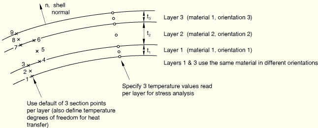
An example of a section with three layers and three integration points per layer is shown in Figure 23.6.5–1.
The material name specified for each layer refers to a material definition (“Material data definition,” Section 16.1.2). The material behavior can be linear or nonlinear.
The orientation for each layer is specified by either the name of the orientation (“Orientations,” Section 2.2.5) associated with the layer or the orientation angle in degrees for the layer. This orientation angle, ![]() , is measured positive counterclockwise around the normal and relative to the overall section orientation, where
, is measured positive counterclockwise around the normal and relative to the overall section orientation, where ![]() . If either of the two local directions from the overall section orientation is not in the surface of the shell,
. If either of the two local directions from the overall section orientation is not in the surface of the shell, ![]() is applied after the section orientation has been projected onto the shell surface. If you do not specify an overall section orientation,
is applied after the section orientation has been projected onto the shell surface. If you do not specify an overall section orientation, ![]() is measured relative to the default local shell directions (see “Conventions,” Section 1.2.2).
is measured relative to the default local shell directions (see “Conventions,” Section 1.2.2).
You must associate the section properties with a region of your model.
| Input File Usage: | *SHELL SECTION, ELSET=name, COMPOSITE, ORIENTATION=name |
where the ELSET parameter refers to a set of shell elements. |
| ABAQUS/CAE Usage: | Property module: |
Simpson's rule and Gauss quadrature are provided to calculate the cross-sectional behavior of a shell. You can specify the number of integration points through the thickness of each layer and the integration method as described below. The default integration method is Simpson's rule with five points for a homogeneous section and Simpson's rule with three points in each layer for a composite section.
The three-point Simpson's rule and the two-point Gauss quadrature are exact for linear problems. The default number of integration points should be sufficient for routine thermal-stress calculations and nonlinear applications (such as predicting the response of an elastic-plastic shell up to limit load). For more severe thermal shock cases or for more complex nonlinear calculations involving strain reversals, more integration points may be required; normally no more than nine integration points (using Simpson's rule) are required. Gaussian integration normally requires no more than five integration points.
Gauss quadrature provides greater accuracy than Simpson's rule when the same number of integration points are used. Therefore, to obtain comparable levels of accuracy, Gauss quadrature requires fewer integration points than Simpson's rule does and, thus, requires less computational time and storage space.
By default, Simpson's rule will be used for the shell section integration. The default number of integration points is five for a homogeneous section and three in each layer for a composite section.
Simpson's integration rule should be used if results output on the shell surfaces or transverse shear stress at the interface between two layers of a composite shell is required and must be used for heat transfer and coupled temperature-displacement shell elements.
| Input File Usage: | *SHELL SECTION, SECTION INTEGRATION=SIMPSON |
| ABAQUS/CAE Usage: | Property module: Create Section: select Shell as the section Category and Homogeneous or Composite as the section Type: Section integration: During analysis, Basic: Thickness integration rule: Simpson |
If you use Gauss quadrature for the shell section integration, the default number of integration points is three for a homogeneous section and two in each layer for a composite section.
In Gauss quadrature there are no integration points on the shell surfaces; therefore, Gauss quadrature should be used only in cases where results on the shell surfaces are not required.
Gauss quadrature cannot be used for heat transfer and coupled temperature-displacement shell elements.
| Input File Usage: | *SHELL SECTION, SECTION INTEGRATION=GAUSS |
| ABAQUS/CAE Usage: | Property module: Create Section: select Shell as the section Category and Homogeneous or Composite as the section Type: Section integration: During analysis: Basic: Thickness integration rule: Gauss |
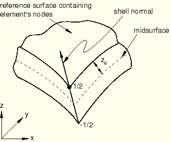
You can define the distance (measured as a fraction of the shell's thickness) from the shell's midsurface to the reference surface containing the element's nodes (see “Defining the initial geometry of conventional shell elements,” Section 23.6.3). Positive values of the offset are in the positive normal direction (see “Shell elements: overview,” Section 23.6.1). When the offset is set equal to 0.5, the top surface of the shell is the reference surface. When the offset is set equal to –0.5, the bottom surface is the reference surface. The default offset is 0, which indicates that the middle surface of the shell is the reference surface.
You can specify an offset value that is greater in magnitude than 0.5. However, this technique should be used with caution in regions of high curvature. All kinematic quantities, including the element's area, are calculated relative to the reference surface, which may lead to a surface area integration error, affecting the stiffness and mass of the shell.
An offset to the shell's top surface is illustrated in Figure 23.6.5–2. The shell offset value is ignored for continuum shell elements.
You can define offsets for homogeneous conventional shells on an element-by-element basis with an element property assignment. See “Assigning element properties on an element-by-element basis,” Section 21.1.5, for details.
| Input File Usage: | Use the following option to specify a value for the shell offset: |
*SHELL SECTION, OFFSET=offset The OFFSET parameter accepts a value or a label (SPOS or SNEG). Specifying SPOS is equivalent to specifying a value of 0.5; specifying SNEG is equivalent to specifying a value of –0.5. |
| ABAQUS/CAE Usage: | Property module: Assign |
You can define a conventional shell with continuously varying thickness by specifying the thickness of the shell at the nodes. The thickness of continuum shell elements is defined by the element geometry.
If you indicate that the nodal thicknesses will be specified, for homogeneous shells any constant shell thickness you specify will be ignored, and the shell thickness will be interpolated from the nodes. The thickness must be defined at all nodes connected to the element.
For composite shells the total thickness is interpolated from the nodes, and the constant layer thicknesses you specify are scaled proportionally such that the sum of the layer thicknesses is equal to the total thickness.
You can define thicknesses for homogeneous conventional shells on an element-by-element basis with an element property assignment. See “Assigning element properties on an element-by-element basis,” Section 21.1.5, for details.
| Input File Usage: | Use both of the following options: |
*NODAL THICKNESS *SHELL SECTION, NODAL THICKNESS |
| ABAQUS/CAE Usage: | Continuously varying shell thicknesses are not supported in ABAQUS/CAE. |
In the finite-membrane-strain shell elements in ABAQUS/Standard and in all shell elements in ABAQUS/Explicit (see “Choosing a shell element,” Section 23.6.2) ABAQUS allows for a possible uniform change in the shell thickness based either on the element material definition or on a specified effective section Poisson's ratio. Thickness change is considered only in geometrically nonlinear analysis (see “General and linear perturbation procedures,” Section 6.1.2).
For conventional shell elements you can specify a value for the effective Poisson's ratio for the section to cause a thickness direction strain under plane stress conditions to be a linear function of the membrane strains. This value must be between –1.0 and 0.5. A value of 0.5 will enforce incompressible behavior of the element in response to membrane strains; a value of 0.0 will enforce constant shell thickness; and a negative value will result in an increase in the shell thickness in response to tensile membrane strains.
Alternatively, you can cause the shell thickness to change based on the element initial elastic material definition, or in ABAQUS/Explicit you can cause the thickness direction strain under plane stress conditions to be a function of the membrane strains and the (nonlinear) material properties.
In ABAQUS/Standard the default is a section Poisson's ratio of 0.5; in ABAQUS/Explicit the default is to base the thickness change on the material definition. See “Finite-strain shell element formulation,” Section 3.6.5 of the ABAQUS Theory Manual, for details regarding the underlying formulation.
| Input File Usage: | Use the following option to specify a value for the effective Poisson's ratio: |
*SHELL SECTION, POISSON= Use the following option to cause the shell thickness to change based on the element initial elastic material definition: *SHELL SECTION, POISSON=ELASTIC Use the following option (available only in ABAQUS/Explicit) to cause the thickness direction strain under plane stress conditions to be a function of the membrane strains and the in-plane material properties: *SHELL SECTION, POISSON=MATERIAL |
| ABAQUS/CAE Usage: | Property module: Create Section: select Shell as the section Category and Homogeneous or Composite as the section Type: Section integration: During analysis: Advanced: Section Poisson's ratio: Use analysis default or Specify value: |
You cannot specify a shell thickness direction behavior based on the initial elastic material definition in ABAQUS/CAE. |
For continuum shell elements the thickness direction strain is computed from the element nodal displacements, which in turn depend on the effective thickness modulus and the section Poisson's ratio. Specifying a section Poisson's ratio causes a thickness direction strain under plane stress conditions to be a linear function of the membrane strains. The stress in the thickness direction is computed from the effective thickness modulus and the effective strain in the thickness direction (thickness direction strain computed from the nodal displacements minus the thickness direction strain under plane stress conditions due to membrane effects). The stress in the thickness direction is computed at the element center and is assumed to be constant through the thickness.
You can choose to precalculate an effective thickness modulus and section Poisson's ratio based on the initial elastic material properties, as defined by the initial temperatures and predefined field variables evaluated at the midpoint of each material layer. The effective thickness modulus is not recalculated during the analysis. Alternatively, you can specify the effective thickness modulus and section Poisson's ratio directly to define the thickness elasticity assuming a homogeneous section. The latter method must be used to define the thickness response if the material properties are unavailable during the preprocessing stage of input; for example, when the material behavior is defined by user subroutine UMAT or VUMAT. By default, the effective thickness modulus is twice the initial in-plane shear modulus based on the material definition. In ABAQUS/Standard the default section Poisson's ratio is 0.5; in ABAQUS/Explicit the default section Poisson's ratio is based on the material definition.
| Input File Usage: | Use the following option to define an effective thickness modulus directly: |
*SHELL SECTION, THICKNESS MODULUS= Use the following option to specify a value for the effective section Poisson's ratio: *SHELL SECTION, POISSON= Use the following option to cause the shell thickness to change based on the element initial elastic material definition: *SHELL SECTION, POISSON=ELASTIC Use the following option (available only in ABAQUS/Explicit) to cause the shell thickness to change based on the element (nonlinear) material definition: *SHELL SECTION, POISSON=MATERIAL |
| ABAQUS/CAE Usage: | Property module: Create Section: select Shell as the section Category and Homogeneous or Composite as the section Type: Section integration: During analysis: Advanced: Section Poisson's ratio: Use analysis default to base the thickness properties on the element material definition or Specify value: |
You cannot specify a shell thickness direction behavior based on the initial elastic material definition in ABAQUS/CAE. |
You can provide nondefault values of the transverse shear stiffness. You must specify the transverse shear stiffness in ABAQUS/Standard if the section is used with shear flexible shells and the material definitions used in the shell section do not include linear elasticity (“Linear elastic behavior,” Section 17.2.1). See “Shell section behavior,” Section 23.6.4, for more information about transverse shear stiffness.
If you do not specify the transverse shear stiffness values, ABAQUS will integrate through the section to determine them. The transverse shear stiffness is precalculated based on the initial elastic material properties, as defined by the initial temperature and predefined field variables evaluated at the midpoint of each material layer. This stiffness is not recalculated during the analysis.
For most shell sections, including layered composite or sandwich shell sections, ABAQUS will calculate the transverse shear stiffness values required in the element formulation. You can override these default values. The default shear stiffness values are not calculated in some cases if estimates of shear moduli are unavailable during the preprocessing stage of input; for example, when the material behavior is defined by user subroutine UMAT, UHYPEL, UHYPER, or VUMAT. You must define the transverse shear stiffnesses in such cases except for STRI3 elements.
| Input File Usage: | Use both of the following options: |
*SHELL SECTION *TRANSVERSE SHEAR STIFFNESS |
| ABAQUS/CAE Usage: | Property module: Create Section: select Shell as the section Category and Homogeneous or Composite as the section Type: Section integration: During analysis: Advanced: toggle on Specify transverse shear |
In ABAQUS/Explicit you can specify second-order accuracy in the shell element formulation. See “Section controls,” Section 21.1.4, for more information.
| Input File Usage: | *SHELL SECTION, CONTROLS=name |
| ABAQUS/CAE Usage: | Mesh module: Mesh |
You can specify a nondefault hourglass control formulation or scale factors for elements that use reduced integration. See “Section controls,” Section 21.1.4, for more information.
In ABAQUS/Standard the nondefault enhanced hourglass control formulation is available only for S4R and SC8R elements. When the enhanced hourglass control formulation is used with composite shells, the average value of the bulk material properties and the minimum value of the shear material properties over all the layers are used for computing the hourglass forces and moments.
In ABAQUS/Standard you can modify the default values for hourglass control stiffness based on the default total stiffness approach for elements that use reduced integration and define a scaling factor for the stiffness associated with the drill degree of freedom (rotation about the surface normal) for elements that use six degrees of freedom at a node.
The stiffness associated with the drill degree of freedom is the average of the direct components of the transverse shear stiffness multiplied by a scaling factor. In most cases the default scaling factor is appropriate for constraining the drill rotation to follow the in-plane rotation of the element. If an additional scaling factor is defined, the additional scaling factor should not increase or decrease the drill stiffness by more than a factor of 100.0 for most typical applications. Usually, a scaling factor between 0.1 and 10.0 is appropriate. Continuum shell elements do not use a drill stiffness; hence, the scale factor is ignored.
There are no hourglass stiffness factors or scale factors for hourglass stiffness for the nondefault enhanced hourglass control formulation. You can define the scale factor for the drill stiffness for the nondefault enhanced hourglass control formulation.
| Input File Usage: | Use both of the following options to specify a nondefault hourglass control formulation or scale factors for reduced-integration elements: |
*SECTION CONTROLS, NAME=name
*SHELL SECTION, CONTROLS=name
Use both of the following options in ABAQUS/Standard to modify the default values for hourglass control stiffness based on the default total stiffness approach for reduced-integration elements and to define a scaling factor for the stiffness associated with the drill degree of freedom (rotation about the surface normal) for six degree of freedom elements: *SHELL SECTION *HOURGLASS STIFFNESS |
| ABAQUS/CAE Usage: | Mesh module: Mesh |
You can specify temperatures and field variables for conventional shell elements by defining the value at the reference surface of the shell and the gradient through the shell thickness or by defining the values at equally spaced points through each layer of the shell's thickness. You can specify a temperature gradient only for elements without temperature degrees of freedom. The temperatures and field variables for continuum shell elements are defined at the nodes and then interpolated to the section points.
The actual values of the temperatures and field variables are specified as either predefined fields or initial conditions (see “Predefined fields,” Section 27.6.1, or “Initial conditions,” Section 27.2.1).
If temperature is to be read as a predefined field from the results file or the output database file of a previous analysis, the temperature must be defined at equally spaced points through each layer of the thickness. In addition, the results file must be modified so that the field variable data are stored in record 201. See “Predefined fields,” Section 27.6.1, for additional details.
You can define the temperature or predefined field by its magnitude on the reference surface of the shell and the gradient through the thickness. If only one value is given, the magnitude will be constant through the thickness.
| Input File Usage: | Use the following option to specify that the temperatures or predefined fields are defined by a gradient: |
*SHELL SECTION Use any of the following options to specify the actual values of the temperatures or predefined fields: *TEMPERATURE *FIELD *INITIAL CONDITIONS, TYPE=TEMPERATURE *INITIAL CONDITIONS, TYPE=FIELD |
| ABAQUS/CAE Usage: | Property module: Create Section: select Shell as the section Category and Homogeneous or Composite as the section Type: Section integration: During analysis: Advanced: Temperature variation: Linear through thickness |
Only initial temperatures and predefined temperature fields are supported in ABAQUS/CAE. Load module: Create Predefined Field: Step: initial_step or analysis_step: choose Other for the Category and Temperature for the Types for Selected Step |
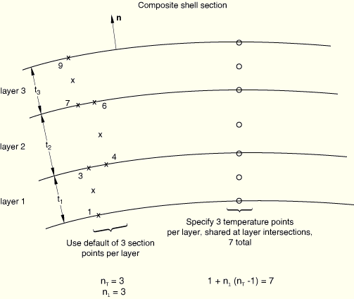
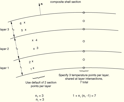
Alternatively, you can define the temperature and field variable values at equally spaced points through the thickness of a shell or of each layer of a composite shell.
For a sequentially coupled thermal-stress analysis in ABAQUS/Standard, the number (n) of equally spaced points through the thickness of a layer is an odd number when temperature values are obtained from the results file or the output database file generated by a previous ABAQUS/Standard heat transfer analysis (since only Simpson's rule can be used for integration through the section in heat transfer analysis). n may be even or odd if the values are supplied from some other source. In either case ABAQUS/Standard interpolates linearly between the two closest defined temperature points to find the temperature values at the section points.
The number of predefined field points through each layer, n, must be the same as the number of integration points used through the same layer in the analysis from which the temperatures are obtained. This requirement implies that in the previous analysis each of the layers must have the same number of integration points.
You specify ![]() temperature or field variable values, where
temperature or field variable values, where ![]() is the number of layers in the shell section and
is the number of layers in the shell section and ![]() (
(![]() > 1) is the value of n. For
> 1) is the value of n. For ![]() =1, you specify
=1, you specify ![]() temperature or field variable values for a given node or node set.
temperature or field variable values for a given node or node set.
| Input File Usage: | Use the following option to specify that the temperatures or predefined fields are defined at equally spaced points: |
*SHELL SECTION, TEMPERATURE=n Use any of the following options to specify the actual values of the temperatures or predefined fields: *TEMPERATURE *FIELD *INITIAL CONDITIONS, TYPE=TEMPERATURE *INITIAL CONDITIONS, TYPE=FIELD |
| ABAQUS/CAE Usage: | Property module: Create Section: select Shell as the section Category and Homogeneous or Composite as the section Type: Section integration: During analysis: Advanced: Temperature variation: Piecewise linear over n values |
Only initial temperatures and predefined temperature fields are supported in ABAQUS/CAE. Load module: Create Predefined Field: Step: initial_step or analysis_step: choose Other for the Category and Temperature for the Types for Selected Step |
An example of this scheme is illustrated in Figure 23.6.5–3 and Figure 23.6.5–4.
The following ABAQUS/Standard heat transfer shell section definition corresponds to this example:*SHELL SECTION, COMPOSITEThis creates degrees of freedom 11–17 in the heat transfer analysis. Temperatures corresponding to these degrees of freedom are then read into the stress analysis at the temperature points shown and interpolated to the section points shown., 3, MAT1, ORI1
, 3, MAT2, ORI2
, 3, MAT3, ORI3
In ABAQUS/Standard if an element with temperature degrees of freedom other than a shell abuts the bottom surface of a shell element with temperature degrees of freedom, the temperature field is made continuous when the elements share nodes. If another element with temperature degrees of freedom abuts the top surface, separate nodes must be used and a linear constraint equation (“Linear constraint equations,” Section 28.2.1) must be used to constrain the temperatures to be the same (that is, to give the same value to the top surface degree of freedom on the shell and degree of freedom 11 on the other element).
For the same reason you must be careful if a different number of temperature points is used in adjacent shell elements. For compatibility MPCs (“General multi-point constraints,” Section 28.2.2) or equation constraints are also needed in this case.
In an ABAQUS/Standard stress analysis temperature output at the section points can be obtained using the element variable TEMP.
If the temperature values were specified at equally spaced points through the thickness, output at the temperature points can be obtained in an ABAQUS/Standard stress analysis, as in a heat transfer analysis, by using the nodal variable NTxx. The nodal variable NTxx should not be used for output at the temperature points with the default gradient method. In this case output variable NT should be requested; NT11 (the reference temperature value) and NT12 (the temperature gradient) will be output automatically.
Other output variables that are relevant for shells are listed in each of the library sections describing the specific shell elements. For example, stresses, strains, section forces and moments, average section stresses, section strains, etc. can be output. The section moments are calculated relative to the reference surface.