
Products: ABAQUS/Standard ABAQUS/Explicit ABAQUS/CAE
This section describes how to specify the values of the following types of predefined fields during an analysis:
temperature,
field variables,
equivalent pressure stress, and
mass flow rate.
Temperature, field variables, equivalent pressure stress, and mass flow rate are time-dependent, predefined (not solution-dependent) fields that exist over the spatial domain of the model. They can be defined:
by entering the data directly,
by reading an ABAQUS results file generated during a previous analysis (usually an ABAQUS/Standard heat transfer analysis), or
in an ABAQUS/Standard user subroutine.
Field variables can also be made solution dependent, which allows you to introduce additional nonlinearities in the ABAQUS material models.
In stress/displacement analysis the temperature difference between a predefined temperature field and any initial temperatures (“Initial conditions,” Section 27.2.1) will create thermal strains if a thermal expansion coefficient is given for the material (“Thermal expansion,” Section 20.1.2). The predefined temperature field also affects temperature-dependent material properties, if any. In ABAQUS/Explicit temperature-dependent material properties may cause longer run times than constant properties.
You define the magnitude and time variation of temperature at the nodes, and ABAQUS interpolates the temperatures to the material points.
| Input File Usage: | Use the following option to specify a predefined temperature field: |
*TEMPERATURE |
| ABAQUS/CAE Usage: | Load module: Create Predefined Field: Step: analysis_step: choose Other for the Category and Temperature for the Types for Selected Step |
Do not specify predefined temperature fields in a pure heat transfer analysis, a coupled thermal-electrical analysis, or a fully coupled temperature-displacement analysis; instead, specify a boundary condition (“Boundary conditions,” Section 27.3.1) to prescribe temperature degrees of freedom (11, 12, ...).
Predefined temperature fields cannot be specified in an adiabatic analysis step or in any mode-based dynamic analysis step.
To specify a predefined temperature field in a restart analysis, the corresponding predefined field must have been specified in the original analysis as either initial temperatures (see “Defining initial temperatures” in “Initial conditions,” Section 27.2.1) or a predefined temperature field.
The usage and treatment of predefined field variables is exactly analogous to that of temperature. An example of a field variable is an electromagnetic field. ABAQUS has no way of solving for such a field; rather, you can prescribe the magnitude and time variation of the field at all of the nodes of the model, and ABAQUS will interpolate the values to the material points.
When prescribing field variable values, you must specify the field variable number being defined; the default is field variable number 1. Field variables must be numbered consecutively starting from one. Repeat the field variable definition to define more than one field variable.
Field variables are mainly used to change material properties depending on the field's value. For example, suppose that you wish to vary Young's modulus linearly between 30 × 106 and 35 × 106 during the response. The linear elastic material definition shown in Table 27.6.1–1could be used.
Table 27.6.1–1 Sample material definition.
| Number of field variable dependencies: 1 | ||
| Young's modulus | Poisson's ratio | Value of field variable 1 |
| 30.E6 | 0.3 | 1.0 |
| 35.E6 | 0.3 | 2.0 |
Field variables can also be used to vary real properties in space by making the properties depend on field variables, as above, and by assigning different field variable values to different nodes.
Making properties depend on field variables will increase the computer time required, since ABAQUS must perform the necessary table look-ups.
| Input File Usage: | Use the following option to specify a predefined field variable: |
*FIELD, VARIABLE=n |
| ABAQUS/CAE Usage: | Predefined field variables are not supported in ABAQUS/CAE. |
To specify a predefined field variable in a restart analysis, the corresponding predefined field must have been specified in the original analysis as either an initial field variable value (see “Defining initial values of predefined field variables” in “Initial conditions,” Section 27.2.1) or a predefined field variable.
You can apply equivalent pressure stress as a predefined field in a mass diffusion analysis. The usage and treatment of pressure stresses is analogous to that of temperatures and field variables. In ABAQUS equivalent pressure stresses are positive when they are compressive.
| Input File Usage: | Use the following option to specify a predefined equivalent pressure stress field: |
*PRESSURE STRESS |
| ABAQUS/CAE Usage: | Predefined equivalent pressure stress is not supported in ABAQUS/CAE. |
Predefined equivalent pressure stress fields can be specified only in a mass diffusion procedure (see “Mass diffusion analysis,” Section 6.8.1).
To specify a predefined equivalent pressure stress field in a restart analysis, the corresponding predefined field must have been specified in the original analysis as either initial pressure stresses (see “Defining initial pressure stress in a mass diffusion analysis” in “Initial conditions,” Section 27.2.1) or a predefined equivalent pressure stress field.
You can specify the mass flow rate per unit area (or through the entire section for one-dimensional elements) for forced convection/diffusion elements in a heat transfer analysis. The usage and treatment of mass flow rate is analogous to that of temperatures and field variables.
| Input File Usage: | Use the following option to specify a predefined mass flow rate field: |
*MASS FLOW RATE |
| ABAQUS/CAE Usage: | Predefined mass flow rate is not supported in ABAQUS/CAE. |
A predefined mass flow rate field can be specified only with forced convection/diffusion elements in a heat transfer procedure (see “Uncoupled heat transfer analysis,” Section 6.5.2).
To specify a predefined mass flow rate field in a restart analysis, the corresponding predefined field must have been specified in the original analysis by using either initial mass flow rates (see “Defining initial mass flow rates in forced convection heat transfer elements” in “Initial conditions,” Section 27.2.1) or a predefined mass flow rate field.
An ABAQUS/Standard results file can be used to specify initial values of temperature, field variables, and pressure stress (see “Initial conditions,” Section 27.2.1). Field variable values must be read from the temperature record (see below). The part (.prt) file from the original analysis is also required when reading data from the results file.
If the zero increment results were requested as output to the ABAQUS/Standard results file (see “Obtaining results at the beginning of a step” in “Output,” Section 4.1.1), you can define initial values of prescribed fields as those existing at the beginning of a step (the zero increment) in the previous heat transfer analysis (field variables and temperatures) or stress/displacement analysis (pressure stress). The .fil file extension is optional.
| Input File Usage: | Use one of the following options: |
*INITIAL CONDITIONS, TYPE=TEMPERATURE, FILE=file, STEP=step, INC=inc *INITIAL CONDITIONS, TYPE=FIELD, VARIABLE=n, FILE=file, STEP=step, INC=inc *INITIAL CONDITIONS, TYPE=PRESSURE STRESS, FILE=file, STEP=step, INC=inc |
| ABAQUS/CAE Usage: | Load module: Create Predefined Field: Step: Initial: choose Other for the Category and Temperature for the Types for Selected Step: select region: Distribution: From results or output database file, File name: file, Step: step, and Increment: inc |
Initial field variables and pressure stress are not supported in ABAQUS/CAE. |
An ABAQUS/Standard output database file can be used to specify initial values of temperature (see “Defining initial temperatures” in “Initial conditions,” Section 27.2.1). The part (.prt) file from the original analysis is also required when reading data from the output database file. Temperature values can be read between dissimilar meshes, as described in “Interpolating initial temperatures for dissimilar meshes from a user-specified results or output database file” in “Initial conditions,” Section 27.2.1.
| Input File Usage: | *INITIAL CONDITIONS, TYPE=TEMPERATURE, FILE=file.odb, STEP=step, INC=inc |
| ABAQUS/CAE Usage: | Load module: Create Predefined Field: Step: Initial: choose Other for the Category and Temperature for the Types for Selected Step: select region: Distribution: From results or output database file, File name: file, Step: step, and Increment: inc |
The prescribed magnitude of a field can vary with time during a step according to an amplitude function. See “Prescribed conditions: overview,” Section 27.1.1, and “Amplitude curves,” Section 27.1.2, for details.
| Input File Usage: | Use one of the following options: |
*TEMPERATURE, AMPLITUDE=amplitude_name *FIELD, AMPLITUDE=amplitude_name *PRESSURE STRESS, AMPLITUDE=amplitude_name *MASS FLOW RATE, AMPLITUDE=amplitude_name |
| ABAQUS/CAE Usage: | In ABAQUS/CAE only predefined temperature fields are available. |
Load module: Create Predefined Field: Step: analysis_step: choose Other for the Category and Temperature for the Types for Selected Step: select region: Distribution: Direct specification or select an analytical field, Amplitude: amplitude_name |
By default, all fields defined in the previous general analysis step remain unchanged in the subsequent general step or in subsequent consecutive linear perturbation steps. Fields do not propagate between linear perturbation steps. You define the fields in effect for a given step relative to the preexisting fields. At each new step the existing fields can be modified and additional fields can be specified. If you specify additional values for a field, the definition of the field will be extended to those nodes where it was previously undefined. Alternatively, you can release all previously applied fields of a given type in a step and specify new ones. In this case any fields of that type that are to be retained must be respecified.
By default, when you modify existing temperatures, field variables, pressure stresses, or mass flow rates, all existing values of the field remain.
| Input File Usage: | Use one of the following options to modify an existing field or to specify an additional field: |
*TEMPERATURE, OP=MOD *FIELD, OP=MOD *PRESSURE STRESS, OP=MOD *MASS FLOW RATE, OP=MOD |
| ABAQUS/CAE Usage: | In ABAQUS/CAE only predefined temperature fields are available. |
Load module: Create Predefined Field or Predefined Field Manager: Edit |
A field that is removed is reset to the value given as an initial condition or to zero if no initial condition was defined. When fields are reset to their initial conditions, the amplitude referred to in the field definition does not apply. In ABAQUS/Standard the amplitude variation defined for the step governs the behavior; in most ABAQUS/Standard procedures the default is to ramp the fields back to their initial conditions (see “Procedures: overview,” Section 6.1.1). In ABAQUS/Explicit the values are always ramped linearly over the step back to their initial conditions.
If the temperatures, field variables, pressure stresses, or mass flow rates are reset to a new value (not to their initial conditions), the amplitude referred to in the field definition applies.
If you choose to remove any field in a step, no fields of that type will be propagated from the previous general step. All fields of the same type that are in effect during this step must be respecified.
| Input File Usage: | Use one of the following options to release all previously applied fields of a particular type and to specify new fields: |
*TEMPERATURE, OP=NEW
*FIELD, OP=NEW
*PRESSURE STRESS, OP=NEW
*MASS FLOW RATE, OP=NEW
If the OP=NEW parameter is used on any field option in a step, it must be used on all field options of the same type within the step. |
| ABAQUS/CAE Usage: | Use the following option to reset a temperature field to the value prescribed in the initial step (or to zero if no initial value was defined): |
Load module: temperature field editor: Reset to initial |
The data for predefined temperature, field variables, pressure stress, or mass flow rate can be contained in a separate input file (see “Input syntax rules,” Section 1.2.1).
| Input File Usage: | Use one of the following options: |
*TEMPERATURE, INPUT=file_name
*FIELD, INPUT=file_name
*PRESSURE STRESS, INPUT=file_name
*MASS FLOW RATE, INPUT=file_name
If the INPUT parameter is omitted, it is assumed that the data lines follow the keyword line. |
| ABAQUS/CAE Usage: | You cannot read field data from a separate input file in ABAQUS/CAE. |
Nodal temperatures calculated during an ABAQUS/Standard heat transfer or coupled thermal-electrical analysis can be used to define temperatures or field variables in a subsequent analysis. The temperatures must have been written to the results or output database file.
In ABAQUS/Standard equivalent pressure stresses calculated during a mechanical analysis can be used in a subsequent mass diffusion analysis if the element output variable SINV was written to the results file averaged at the nodes (see “Element output” in “Output to the data and results files,” Section 4.1.2).
Once the data are available in a results file or output database file, they can be read into a subsequent analysis as a predefined field. Data for field variables and pressure stress can be read from a previously generated results file. Data for temperatures can be read from a previously generated results or output database file. Data for temperatures to be interpolated between dissimilar meshes can be read only from the output database file. The part (.prt) file from the original analysis is also required when reading temperature data from the results or output database file.
When the output file of an ABAQUS analysis involving beam and/or shell elements is used to define temperatures, you must ensure that the number of temperature points through the section defined for corresponding elements is consistent between the two analyses. Inconsistent temperature point definition will result in an incorrect transfer of prescribed field quantities.
To read field values from a user-specified results file, the data must have been written to the results file as nodal output (see “Node output” in “Output to the data and results files,” Section 4.1.2). Only nodal quantities can be read from the results file. Since field variables can be written to the results file only as element quantities (record key 9), they cannot be read directly into a subsequent analysis. In this case you must generate a results file with the field data in the temperature record, even if the field variable in the current analysis is the same as a field variable in the previous analysis. Multiple results files must be generated for multiple field variables.
To generate the results file, you can write a program to create a results file (without running an ABAQUS analysis) according to the format described in Chapter 5, “File Output Format.” Examples of such programs are shown in that chapter. If the values will be read in as temperatures or field variables, the data must be written as nodal quantities with record key 201. If the values will be read in as a pressure stress field, the data must be averaged at the nodes (as explained in “Output to the data and results files,” Section 4.1.2) and written as record key 12.
You must specify the name of the results file from which the data are to be read for a temperature, field variable, or pressure stress. The .fil file extension is optional. If both .fil and .odb files exist for a temperature field and no extension is specified, the results file will be used.
| Input File Usage: | *TEMPERATURE, FILE=file *FIELD, FILE=file *PRESSURE STRESS, FILE=file |
| ABAQUS/CAE Usage: | Load module: Create Predefined Field: Step: analysis_step: choose Other for the Category and Temperature for the Types for Selected Step: select region: Distribution: From results or output database file, File name: file |
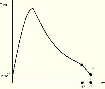
In a direct cyclic analysis in ABAQUS/Standard the temperature values must be cyclic over the step: the start value must be equal to the end value. To create a cyclic temperature history from a prior heat transfer analysis that is not cyclic, you can set the starting time, f (measured relative to the total step time period, ![]() ), after which the temperatures read from the results file will be ramped back to their initial condition values. At any time point
), after which the temperatures read from the results file will be ramped back to their initial condition values. At any time point ![]() , the temperature value is equal to
, the temperature value is equal to
![]()
Figure 27.6.1–1 Ramp temperatures to their initial condition values after ![]() to create a cyclic temperature history.
to create a cyclic temperature history.
| Input File Usage: | Use the following option to set the starting time for a cyclic temperature history: |
*TEMPERATURE, FILE=file, BTRAMP=f |
| ABAQUS/CAE Usage: | Cyclic temperature histories are not supported in ABAQUS/CAE. |
To read temperature values from a user-specified output database file, the temperatures must have been written to the output database file as nodal output (see “Node output” in “Output to the output database,” Section 4.1.3).
You must specify the name of the output database file from which the data are to be read for a temperature field. The .odb extension must be included if both results and output database files exist.
| Input File Usage: | *TEMPERATURE, FILE=file |
| ABAQUS/CAE Usage: | Load module: Create Predefined Field: Step: analysis_step: choose Other for the Category and Temperature for the Types for Selected Step: select region: Distribution: From results or output database file, File name: file |
Sequentially coupled thermal-stress analysis can be performed between the same meshes, between meshes that differ only in the element order (first-order element in heat transfer analysis and second-order element in thermal-stress analysis), or between dissimilar meshes. To a run sequentially coupled thermal-stress analysis between the same meshes, no additional computations are required. To run a sequentially coupled thermal-stress analysis between meshes that differ only in the element order, you must activate the midside node capability. To run a sequentially coupled thermal-stress analysis between dissimilar meshes, you must activate the general interpolation capability. The midside node capability and the general interpolation capability are mutually exclusive.
In some cases it makes sense to perform an ABAQUS/Standard heat transfer analysis using first-order elements followed by a thermal-stress analysis using second-order elements (and an otherwise similar mesh). For example, a heat transfer analysis including latent heat effects—for which first-order elements are best suited—can be followed by a stress analysis using second-order elements, which generally have superior deformation characteristics. In addition, the first-order temperature field calculated in the heat transfer analysis is consistent with the first-order thermal strain field provided by the second-order stress/displacement elements.
For the instances in which there is a change in the order of interpolation of element temperature variables between the heat transfer analysis and the stress analysis, temperatures must be assigned to the midside nodes of the stress/displacement elements based on the temperatures of the corner nodes of the heat transfer elements. If you specify that the midside node temperatures are needed, ABAQUS will interpolate the temperatures of the midside nodes of the second-order stress/displacement elements from the corner nodes using first-order interpolation. If the midside node capability is activated in cases where both the heat transfer analysis and the stress analysis are performed with second-order elements, it is ignored. One exception is that if variable-node second-order stress/displacement elements are used in the stress analysis, activating the midside node capability will cause ABAQUS to interpolate the temperatures of the midface nodes in the variable node elements from the corner or midside nodes using first-order interpolation.
Since it is assumed that the corner node temperatures have been generated in a previous heat transfer analysis, the midside node capability can be used only when the temperature field values are read from a user-specified results or output database file. You must ensure that the nodal temperatures calculated during the heat transfer analysis are written to the results or output database file. Once the temperatures of the corner nodes are read in the subsequent stress/displacement analysis, ABAQUS interpolates the midside node temperatures so that all nodes have temperatures assigned to them.
You must ensure that all temperatures of the corner nodes belonging to elements for which midside node temperatures are to be interpolated are read from the heat transfer analysis results or output database file. If the corner node temperatures are defined using a mixture of direct data input, reading from the results file or output database file, and user subroutine UTEMP, midside node temperatures that give unrealistic temperature fields may result. In practice, the capability for calculating midside node temperatures is most useful when temperatures generated by a heat transfer analysis are read from the results or output database file for the whole mesh during the stress analysis. Once the midside node capability is activated in a step, the capability will remain active throughout the remainder of the analysis.
Values of temperature for nodes that existed in the original analysis but do not exist in the current analysis will be ignored. Similarly, if additional nodes (but not midside nodes) exist in the current analysis, the values of fields at these nodes cannot be prescribed by reading the output files.
| Input File Usage: | Use the following option to interpolate temperatures between meshes that differ only in the element order: |
*TEMPERATURE, FILE=file, MIDSIDE |
| ABAQUS/CAE Usage: | Load module: Create Predefined Field: Step: analysis_step: choose Other for the Category and Temperature for the Types for Selected Step: select region: Distribution: From results or output database file, File name: file, Mesh compatibility: Compatible, and toggle on Interpolate midside nodes |
In some cases the model for a heat transfer analysis and the model for a thermal-stress analysis may require different meshes; for example, you may want to model a smooth temperature distribution in the heat transfer analysis and stress concentration regions in the thermal-stress analysis. Both meshes have to be different and independent of each other in such cases. ABAQUS offers a general interpolation capability that allows for the use of dissimilar meshes for heat transfer and thermal-stress analyses.
Temperatures can be interpolated between dissimilar meshes only when the temperatures are read from an output database file. If temperatures for nodes in the heat transfer analysis that are needed for interpolation are not written to the output database file, the values at those nodes are assumed to be zero, which may lead to incorrect results for the temperature values in the stress analysis. Similarly, if additional nodes exist in the mesh for the stress analysis, the values of temperatures at these nodes are assumed to be zero. Interpolation of temperatures can also be used for specifying temperature as a field variable in a submodel thermal-stress analysis where the temperature values are read directly from a global heat transfer analysis.
You can specify an interpolation tolerance for use in locating the nodes in the heat transfer analysis. The tolerance can be specified as an absolute value or as a fraction of the average element size. In a multi-step thermal-stress analysis in which several steps read the temperature values from the same file, ABAQUS interpolates the temperature values only once. If different interpolation tolerance values are used for each step, the interpolation is based on the largest specified tolerance value. If a restart analysis is performed from a particular step in the thermal-stress analysis, the restart interpolation is based on the tolerance value specified for that step.
| Input File Usage: | Use the following option to interpolate temperatures between dissimilar meshes: |
*TEMPERATURE, FILE=file.odb, INTERPOLATE Use the following option to specify the interpolation tolerance as an absolute value: *TEMPERATURE, FILE=file.odb, INTERPOLATE, ABSOLUTE EXTERIOR TOLERANCE=tolerance Use the following option to specify the interpolation tolerance as a fraction of the average element size: *TEMPERATURE, FILE=file.odb, INTERPOLATE, EXTERIOR TOLERANCE=tolerance |
| ABAQUS/CAE Usage: | Load module: Create Predefined Field: Step: analysis_step: choose Other for the Category and Temperature for the Types for Selected Step: select region: Distribution: From results or output database file, File name: file.odb, Mesh compatibility: Incompatible, exterior tolerance: absolute or relative tolerance |
You can specify the first and last step, respectively, from which results will be read. Similarly, you can specify the first and last increment, respectively, from which results will be read. You can specify any combination of these values. Any zero-increment file output that is present in the results file of an ABAQUS/Standard analysis (written only if the zero increment results are requested; see “Obtaining results at the beginning of a step” in “Output,” Section 4.1.1) will be ignored. Results must have been written to the results or output database file at the specified step and increment.
If you do not specify the first step from which to read, ABAQUS will begin reading results from the first step available in the results or output database file.
If you do not specify the first increment from which to read, ABAQUS will begin reading results from the first increment available in the first step from which results will be read (the first increment following the zero increment if zero-increment file output is present in the results file).
If you do not specify the last step from which to read, the first step from which results will be read will also be the last step.
If you do not specify the last increment from which to read, ABAQUS will read the results or output database file until it reaches the last available increment in the last step from which results will be read.
| Input File Usage: | Use one of the following options: |
*TEMPERATURE, FILE=file, BSTEP=bstep, BINC=binc, ESTEP=estep,
EINC=einc
*FIELD, FILE=file, BSTEP=bstep, BINC=binc, ESTEP=estep, EINC=einc
*PRESSURE STRESS, FILE=file, BSTEP=bstep, BINC=binc, ESTEP=estep,
EINC=einc
For example, the following input would read temperature data from output database file heat.odb beginning at Step 2, increment 2, and ending at Step 3, increment 5: *TEMPERATURE, FILE=heat.odb, BSTEP=2, BINC=2, ESTEP=3, EINC=5 |
| ABAQUS/CAE Usage: | Load module: Create Predefined Field: Step: analysis_step: choose Other for the Category and Temperature for the Types for Selected Step: select region: Distribution: From results or output database file, File name: file, Begin step: bstep, Begin increment: binc, End step: estep, and End increment: einc |
When ABAQUS reads temperature, field variable, or equivalent pressure stress data from a results file or temperatures from an output database file, it must obtain values of the field at the time points used by the analysis. Since data corresponding to these time points are usually not present in the results or output database files, ABAQUS will interpolate linearly in time between the time points stored in the file to obtain values at the time points required by the analysis. Since the interpolation is linear, you must take care to provide sufficient data in the results or output database file to make this interpolation meaningful.
For the purpose of such interpolation the time period of the results being read in is taken to start at the beginning of the starting increment (either user-specified or default) and to end at the completion of the ending increment (either user-specified or default).
If the analysis requires data at a time point prior to the first increment for which data are available in the either of files, ABAQUS will interpolate between the given initial condition data and the data of the first increment stored in the file.
If data for multiple fields are being read in the same step and the time values corresponding to the starting step and increment or to the ending step and increment are different for different fields, ABAQUS interpolates through the total time period from the earliest time point chosen in any file to the latest. For example, suppose the starting increment in the starting step in the temperature file begins at 3 sec and the ending increment in the ending step ends at 6 sec. During the same step we also read field variable data, for which the starting increment in the starting step begins at 2 sec and the ending increment in the ending step ends at 5 sec. In such a case the time period used for interpolation is from 2 sec to 6 sec.
It is convenient to set the period of the step equal to the time period of the files being read in. Otherwise, ABAQUS will automatically scale the time period from the results or output database file to match the time period of the stress analysis. The scale factor is ![]() , where
, where ![]() is the time period of the stress analysis and
is the time period of the stress analysis and ![]() is the total time period obtained from all results or output database files, as described above.
is the total time period obtained from all results or output database files, as described above.
In ABAQUS/Standard it is sometimes desirable to carry out a calculation corresponding to the field values at a particular point in time. For example, suppose that temperature data are available in the output file for increment 10 at time ![]() and increment 15 at time
and increment 15 at time ![]() and that you wish to carry out a static analysis based on temperature values at
and that you wish to carry out a static analysis based on temperature values at ![]() . In this case ABAQUS must interpolate linearly between the results at
. In this case ABAQUS must interpolate linearly between the results at ![]() and
and ![]() to obtain the intermediate result at
to obtain the intermediate result at ![]() . To accomplish this task, you should specify an initial time increment of 4.5 and a time period of 5. for the static analysis step and read the temperature values from the output file starting at Step 1, Increment 1 and ending at Step 1, Increment 15. Specifying a starting increment of 1 instead of 10 ensures that
. To accomplish this task, you should specify an initial time increment of 4.5 and a time period of 5. for the static analysis step and read the temperature values from the output file starting at Step 1, Increment 1 and ending at Step 1, Increment 15. Specifying a starting increment of 1 instead of 10 ensures that ![]() is the entire time period stored in the output file, not just the period between increments 10 and 15; hence, the scale factor between the output file data and the static analysis is unity, and the initial time of 4.5 has the desired meaning.
is the entire time period stored in the output file, not just the period between increments 10 and 15; hence, the scale factor between the output file data and the static analysis is unity, and the initial time of 4.5 has the desired meaning.
To track initial transients accurately, ABAQUS/Standard may automatically reduce the initial time increment for the step. If the user-specified suggested initial time increment is greater than the scaled value of the first time increment read from the ABAQUS/Standard results file, ABAQUS/Standard will use that scaled value.
Temperatures and field variables cannot be read from a user-specified file in a modified Riks static analysis step (“Unstable collapse and postbuckling analysis,” Section 6.2.4).
Temperature cannot be interpolated from a coupled thermal-electrical analysis.
Equivalent pressure stress cannot be read from the results file if the model is defined in terms of an assembly of part instances.
Field variables and pressure stress cannot be read from the output database file.
In ABAQUS/Standard you can specify predefined temperatures, field variables, equivalent pressure stresses, or mass flow rates at the nodes in a user subroutine. Temperature values can be defined in user subroutine UTEMP; field variable values, in user subroutine UFIELD; equivalent pressure stress values, in user subroutine UPRESS; and mass flow rates, in user subroutine UMASFL.
The user subroutine (UTEMP, UFIELD, UPRESS, or UMASFL) will be called for each specified node. Field values entered directly will be ignored. If a results or output database file has been specified in addition to the user subroutine, values read from the results or output database file will be passed into the user subroutine for possible modification.
| Input File Usage: | Use one of the following options: |
*TEMPERATURE, USER *FIELD, USER *PRESSURE STRESS, USER *MASS FLOW RATE, USER |
| ABAQUS/CAE Usage: | Load module: Create Predefined Field: Step: analysis_step: choose Other for the Category and Temperature for the Types for Selected Step: select region: Distribution: User-defined or From results or output database file and user-defined |
If multiple field variables are predefined, only one field variable at a time can be redefined in user subroutine UFIELD. There are situations in which the analysis requires a number of field variables that are predefined with respect to the solution but depend on each other. You can specify the number of field variables to be updated simultaneously at a point, n. ABAQUS/Standard passes information about n field variables at each specified node into UFIELD.
You can update all or part of the field variables used in the analysis but must remember that the field variables are numbered consecutively from 1. If, for example, you have four field variables in the analysis and want to update the second and third variables simultaneously in subroutine UFIELD, you must specify n=3. In this case ABAQUS/Standard passes information about the first three field variables into subroutine UFIELD, and you update only the second and third variables.
| Input File Usage: | *FIELD, USER, NUMBER=n |
| ABAQUS/CAE Usage: | Predefined field variables are not supported in ABAQUS/CAE. |
In ABAQUS/Standard solution-dependent field variables can be defined in user subroutine USDFLD. The values of predefined field variables or initial fields can be passed into user subroutine USDFLD and can be changed in that routine—see “Material data definition,” Section 16.1.2.
Changes to the field variables in USDFLD are local to the material point and do not affect the nodal values.
If both results or output database file input and direct data input are used in the same step, the direct data input will take precedence if both define the field at the same node. If user subroutine input is specified, the values given directly are ignored and the user subroutine modifies the values read from the results or output database file.
It is possible to specify either one or several values of a predefined field at a node, depending on the element type that is used. For solid elements only one value can be given at a node. Since only solid elements can be used in mass diffusion analysis, this is the only way to define equivalent pressure stresses at a node. The following possibilities exist for temperatures and field variables in beam and shell elements:
For shell and beam elements with general cross-section definitions, the temperature and field variable magnitude at points in the section is defined by the value at the reference surface. Any gradient of these variables specified across the section is ignored.
For shell and beam elements with cross-sections that require numerical integration, the temperature and field variable magnitudes at points in the section can be defined either from the value at the reference surface and the gradient or gradients across the section or by giving the values at a number of points across the section. The choice between these two methods is made in the section definition (see “Specifying temperature and field variables” in “Using a shell section integrated during the analysis to define the section behavior,” Section 23.6.5, and “Specifying temperature and field variables” in “Using a beam section integrated during the analysis to define the section behavior,” Section 23.3.6, for details).
See Part VI, “Elements,” for the details of use with each element type. The default, if only one value is given, is a constant magnitude across the section.
ABAQUS assumes that the field definitions (including initial conditions) at all the nodes of any element are compatible with the field definition method chosen for the element. Cases may arise where the definition of a field changes from one element to the next (for example, when two adjacent shell elements have a different number of section points through the thickness or when the temperature and field variable magnitudes for one beam element are defined by giving the values at a number of points across the section while those for the abutting beam element are defined from the value at the reference surface and the gradient or gradients across the section). In these cases separate nodes should be used on the interface between such elements and multi-point constraints should be applied to make the displacements and rotations the same at corresponding nodes (see “General multi-point constraints,” Section 28.2.2); otherwise, the fields on the nodes at the interface will be used for each adjacent element with the field definition method chosen for the element.