Products: ABAQUS/Standard ABAQUS/Explicit ABAQUS/CAE
When surfaces are in contact they usually transmit shear as well as normal forces across their interface. There is generally a relationship between these two force components. The relationship, known as the friction between the contacting bodies, is usually expressed in terms of the stresses at the interface of the bodies. The friction models available in ABAQUS:
include the classical isotropic Coulomb friction model (see “Coulomb friction,” Section 5.2.3 of the ABAQUS Theory Manual), which in ABAQUS:
in its general form allows the friction coefficient to be defined in terms of slip rate, contact pressure, average surface temperature at the contact point, and field variables; and
provides the option for you to define a static and a kinetic friction coefficient with a smooth transition zone defined by an exponential curve;
allow the introduction of a shear stress limit, ![]() , which is the maximum value of shear stress that can be carried by the interface before the surfaces begin to slide;
, which is the maximum value of shear stress that can be carried by the interface before the surfaces begin to slide;
include an anisotropic extension of the basic Coulomb friction model in ABAQUS/Standard;
include a model that eliminates frictional slip when surfaces are in contact;
include a “softened” interface model for sticking friction in ABAQUS/Explicit in which the shear stress is a function of elastic slip;
can be implemented with a stiffness (penalty) method, a kinematic method (in ABAQUS/Explicit), or a Lagrange multiplier method (in ABAQUS/Standard), depending on the contact algorithm used; and
can be defined in user subroutine FRIC (in ABAQUS/Standard) or VFRIC (in ABAQUS/Explicit for the contact pair algorithm only), which allows modeling of very general frictional surface conditions.
ABAQUS assumes by default that the interaction between contacting bodies is frictionless. You can include a friction model in a contact property definition for both surface-based contact and element-based contact.
| Input File Usage: | Use both of the following options for surface-based contact: |
*SURFACE INTERACTION, NAME=interaction_property_name
*FRICTION
Use both of the following options for element-based contact in ABAQUS/Standard: *INTERFACE or *GAP, ELSET=name *FRICTION |
| ABAQUS/CAE Usage: | Interaction module: contact property editor: Mechanical |
Element-based contact is not supported in ABAQUS/CAE. |
The methods used to change friction properties during an analysis differ between ABAQUS/Standard and ABAQUS/Explicit.
It is possible to remove, to modify, or to add a friction model to a contact property definition in any particular step of an ABAQUS/Standard simulation. In some models, such as shrink-fit contact interference problems, friction should not be added until after the first steps have been completed. In other models friction might be removed or lowered to represent the introduction of a lubricant between the bodies.
You must identify which contact property definition or contact element set is being changed.
| Input File Usage: | Use both of the following options for surface-based contact: |
*CHANGE FRICTION, INTERACTION=name
*FRICTION
Use both of the following options for element-based contact: *CHANGE FRICTION, ELSET=name *FRICTION |
| ABAQUS/CAE Usage: | Define a contact property with a new friction definition. Then change the contact property assigned to an interaction in a particular step. |
Interaction module: Contact property editor: Mechanical Interaction editor: Contact interaction property: new_interaction_property_name Element-based contact is not supported in ABAQUS/CAE. |
You can use an amplitude curve (specifying a relative magnitude definition) to define the time variation of the change in friction coefficients throughout the step.
If the friction coefficient is dependent on slip rate, contact pressure, average surface temperature at the contact point, or field variables, the current change in the friction coefficient at a material point is defined as the difference between the friction coefficient for the current slip rate, contact pressure, etc. and the friction coefficient at the end of the previous step, multiplied by the amplitude magnitude.
If you do not specify an amplitude curve, the change in friction coefficients is applied immediately at the beginning of the step or ramped up linearly over the step, depending on the amplitude variation assigned to the step (see “Procedures: overview,” Section 6.1.1). If the friction coefficients are changed from finite values to rough friction or from rough friction to finite values, the change is always applied immediately at the beginning of the step. Changes in any other friction properties, such as the allowable elastic slip, are also applied instantaneously at the start of the step. Use caution when changing the friction model during an analysis if the surfaces using the model are still in contact and carrying loads. Sudden changes in the frictional model in such cases may lead to convergence problems.
| Input File Usage: | *CHANGE FRICTION, AMPLITUDE=name |
| ABAQUS/CAE Usage: | Time-dependent changes in friction coefficients are not supported in ABAQUS/CAE. |
You can reset the frictional properties of the specified contact property definition or element set to their original values.
| Input File Usage: | Use either of the following options: |
*CHANGE FRICTION, RESET, INTERACTION=name
*CHANGE FRICTION, RESET, ELSET=name
In this case the *FRICTION option is not needed. |
| ABAQUS/CAE Usage: | Interaction module: |
Contact property editor: Mechanical Interaction editor: Contact interaction property: default_interaction_property_name |
In ABAQUS/Explicit the friction definition is specified as part of the model definition for a general contact analysis and as part of the history definition for a contact pair analysis. See “Contact properties for general contact,” Section 29.3.3, and “Contact properties for ABAQUS/Explicit contact pairs,” Section 29.4.3, for information on changing aspects of any contact property definition during an ABAQUS/Explicit analysis.
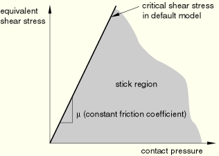
The basic concept of the Coulomb friction model is to relate the maximum allowable frictional (shear) stress across an interface to the contact pressure between the contacting bodies. In the basic form of the Coulomb friction model, two contacting surfaces can carry shear stresses up to a certain magnitude across their interface before they start sliding relative to one another; this state is known as sticking. The Coulomb friction model defines this critical shear stress, ![]() , at which sliding of the surfaces starts as a fraction of the contact pressure, p, between the surfaces (
, at which sliding of the surfaces starts as a fraction of the contact pressure, p, between the surfaces (![]() ). The stick/slip calculations determine when a point transitions from sticking to slipping or from slipping to sticking. The fraction,
). The stick/slip calculations determine when a point transitions from sticking to slipping or from slipping to sticking. The fraction, ![]() , is known as the coefficient of friction.
, is known as the coefficient of friction.
For the case when the slave surface consists of a node-based surface, the contact pressure is equal to the normal contact force divided by the cross-sectional area at the contact node. In ABAQUS/Standard the default cross-sectional area is 1.0; you can specify a cross-sectional area associated with every node in the node-based surface when the surface is defined or, alternatively, assign the same area to every node through the contact property definition. In ABAQUS/Explicit the cross-sectional area is always 1.0, and you cannot change it.
The basic friction model assumes that ![]() is the same in all directions (isotropic friction). For a three-dimensional simulation there are two orthogonal components of shear stress,
is the same in all directions (isotropic friction). For a three-dimensional simulation there are two orthogonal components of shear stress, ![]() and
and ![]() , along the interface between the two bodies. These components act in the slip directions for the contact surfaces or contact elements. The slip directions for contact surfaces are defined in “Contact formulation for ABAQUS/Standard contact pairs,” Section 29.2.2, and those for contact elements are defined in the sections describing contact modeling with those elements.
, along the interface between the two bodies. These components act in the slip directions for the contact surfaces or contact elements. The slip directions for contact surfaces are defined in “Contact formulation for ABAQUS/Standard contact pairs,” Section 29.2.2, and those for contact elements are defined in the sections describing contact modeling with those elements.
ABAQUS combines the two shear stress components into an “equivalent shear stress,” ![]() , for the stick/slip calculations, where
, for the stick/slip calculations, where ![]() . In addition, ABAQUS combines the two slip velocity components into an equivalent slip rate,
. In addition, ABAQUS combines the two slip velocity components into an equivalent slip rate, ![]() . The stick/slip calculations define a surface (see Figure 30.1.5–1 for a two-dimensional representation) in the contact pressure–shear stress space along which a point transitions from sticking to slipping.
. The stick/slip calculations define a surface (see Figure 30.1.5–1 for a two-dimensional representation) in the contact pressure–shear stress space along which a point transitions from sticking to slipping.
There are two ways to define the basic Coulomb friction model in ABAQUS. In the default model the friction coefficient is defined as a function of the equivalent slip rate and contact pressure. Alternatively, you can specify the static and kinetic friction coefficients directly.
In the default model you define the coefficient of friction directly as
![]()
The friction coefficient can depend on slip rate, contact pressure, temperature, and field variables. By default, it is assumed that the friction coefficients do not depend on field variables.
The coefficient of friction can be set to any nonnegative value. A zero friction coefficient means that no shear forces will develop and the contact surfaces are free to slide. You do not need to define a friction model for such a case.
| Input File Usage: | *FRICTION, DEPENDENCIES=n |
| ABAQUS/CAE Usage: | Interaction module: contact property editor: Mechanical |
If necessary, toggle on Use slip-rate-dependent data, Use contact-pressure-dependent data, and/or Use temperature-dependent data; and/or specify the Number of field variable dependencies in addition to slip rate, contact pressure, and temperature. |
Experimental data show that the friction coefficient that opposes the initiation of slipping from a sticking condition is different from the friction coefficient that opposes established slipping. The former is typically referred to as the “static” friction coefficient, and the latter is referred to as the “kinetic” friction coefficient. Typically, the static friction coefficient is higher than the kinetic friction coefficient.
In the default model the static friction coefficient corresponds to the value given at zero slip rate, and the kinetic friction coefficient corresponds to the value given at the highest slip rate. The transition between static and kinetic friction is defined by the values given at intermediate slip rates. In this model the static and kinetic friction coefficients can be functions of contact pressure, temperature, and field variables.
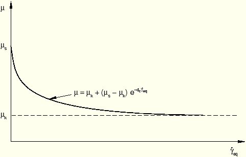
ABAQUS also provides a model to specify a static and a kinetic friction coefficient directly. In this model it is assumed that the friction coefficient decays exponentially from the static value to the kinetic value according to the formula:
![]()
You can provide the static friction coefficient, the kinetic friction coefficient, and the decay coefficient directly (see Figure 30.1.5–2).
| Input File Usage: | *FRICTION, EXPONENTIAL DECAY |
| ABAQUS/CAE Usage: | Interaction module: contact property editor: Mechanical |
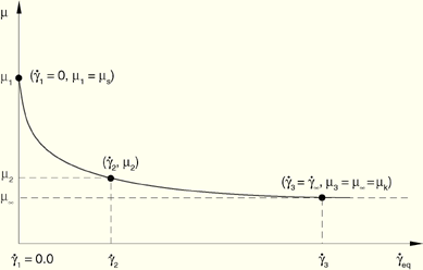
Alternatively, you can provide test data points to fit the exponential model. At least two data points must be provided. The first point represents the static coefficient of friction specified at ![]() , and the second point, (
, and the second point, (![]() ,
, ![]() ) (shown in Figure 30.1.5–3), corresponds to an experimental measurement taken at a reference slip rate
) (shown in Figure 30.1.5–3), corresponds to an experimental measurement taken at a reference slip rate ![]() .
.
| Input File Usage: | *FRICTION, EXPONENTIAL DECAY, TEST DATA |
| ABAQUS/CAE Usage: | Interaction module: contact property editor: Mechanical |
You can specify an optional equivalent shear stress limit, ![]() , so that, regardless of the magnitude of the contact pressure stress, sliding will occur if the magnitude of the equivalent shear stress reaches this value (see Figure 30.1.5–4). A value of zero is not allowed.
, so that, regardless of the magnitude of the contact pressure stress, sliding will occur if the magnitude of the equivalent shear stress reaches this value (see Figure 30.1.5–4). A value of zero is not allowed.
This shear stress limit is typically introduced in cases when the contact pressure stress may become very large (as can happen in some manufacturing processes), causing the Coulomb theory to provide a critical shear stress at the interface that exceeds the yield stress in the material beneath the contact surface. A reasonable upper bound estimate for ![]() is
is ![]() , where
, where ![]() is the Mises yield stress of the material adjacent to the surface; however, empirical data are the best source for
is the Mises yield stress of the material adjacent to the surface; however, empirical data are the best source for ![]() .
.
| Input File Usage: | *FRICTION, TAUMAX= |
| ABAQUS/CAE Usage: | Interaction module: contact property editor: Mechanical |
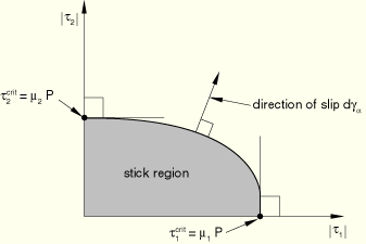
The anisotropic friction model available in ABAQUS/Standard allows for different friction coefficients in the two orthogonal directions on the contact surface. These orthogonal directions coincide with the slip directions defined in “Contact formulation for ABAQUS/Standard contact pairs,” Section 29.2.2; and those for contact elements are described in the sections defining contact modeling with those elements. The orientation of the slip directions cannot be changed.
If you indicate that the anisotropic friction model should be used, you must specify two friction coefficients, where ![]() is the coefficient of friction in the first slip direction and
is the coefficient of friction in the first slip direction and ![]() is the coefficient of friction in the second slip direction.
is the coefficient of friction in the second slip direction.
The critical shear stress surface (see Figure 30.1.5–5) is an ellipse in ![]() –
–![]() space with the two extreme points being
space with the two extreme points being ![]() and
and ![]() . The size of this ellipse will change with the change in contact pressure between the surfaces. The direction of slip,
. The size of this ellipse will change with the change in contact pressure between the surfaces. The direction of slip, ![]() , is orthogonal to the critical shear stress surface.
, is orthogonal to the critical shear stress surface.
The friction coefficient can depend on slip rate, contact pressure, temperature, and field variables. By default, it is assumed that the friction coefficients do not depend on field variables.
| Input File Usage: | *FRICTION, ANISOTROPIC, DEPENDENCIES=n |
| ABAQUS/CAE Usage: | Interaction module: contact property editor: Mechanical |
If necessary, toggle on Use slip-rate-dependent data, Use contact-pressure-dependent data, and/or Use temperature-dependent data; and/or specify the Number of field variable dependencies in addition to slip rate, contact pressure, and temperature. |
ABAQUS offers the option of specifying an infinite coefficient of friction (![]() ). This type of surface interaction is called “rough” friction, and with it all relative sliding motion between two contacting surfaces is prevented. ABAQUS/Standard uses Lagrange multipliers to enforce this constraint; ABAQUS/Explicit uses either a kinematic or penalty method, depending on the contact formulation chosen.
). This type of surface interaction is called “rough” friction, and with it all relative sliding motion between two contacting surfaces is prevented. ABAQUS/Standard uses Lagrange multipliers to enforce this constraint; ABAQUS/Explicit uses either a kinematic or penalty method, depending on the contact formulation chosen.
Rough friction is intended for nonintermittent contact; once surfaces close and undergo rough friction, they should remain closed. Convergence difficulties may arise in ABAQUS/Standard if a closed contact interface with rough friction opens, especially if large shear stresses have developed. The rough friction model is typically used in conjunction with the no separation contact pressure-overclosure relationship for motions normal to the surfaces (see “Using the no separation relationship” in “Contact pressure-overclosure relationships,” Section 30.1.2), which prohibits separation of the surfaces once they are closed.
When rough friction is used with the no separation relationship for hard contact in ABAQUS/Explicit specified with the kinematic contact method, no relative motions of the surfaces will occur. For hard contact in ABAQUS/Explicit specified with the penalty contact method, relative motions will be limited to the elastic slip and penetration corresponding to the inexact satisfaction of the contact constraints by the applied penalty forces. When softened tangential behavior is specified in ABAQUS/Explicit (see “Defining tangential softening in ABAQUS/Explicit” below), the relative surface motions will be governed by the specified softening behavior.
| Input File Usage: | *FRICTION, ROUGH |
| ABAQUS/CAE Usage: | Interaction module: contact property editor: Mechanical |
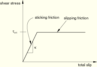
In some cases some incremental slip may occur even though the friction model determines that the current frictional state is “sticking.” In other words, the slope of the shear (frictional) stress versus total slip relationship may be finite while in the “sticking” state, as shown in Figure 30.1.5–6.
The relationship shown in this figure is analogous to elastic-plastic material behavior without hardening:Frictional constraints are enforced with a stiffness (penalty method) by default in ABAQUS/Standard and for the general contact algorithm in ABAQUS/Explicit; in this case the sticking stiffness will have a finite value. An infinite sticking stiffness, in which case the elastic slip is always zero, can be achieved with the optional Lagrange multiplier method for imposing frictional constraints in ABAQUS/Standard or with the kinematic constraint method (available only for contact pairs) in ABAQUS/Explicit. In ABAQUS/Explicit some tangential contact damping acts on the elastic slip rate by default, as discussed in “Contact damping,” Section 30.1.3. Tangential softening to reflect a physical behavior is available only in ABAQUS/Explicit.
To activate softened tangential behavior in ABAQUS/Explicit, specify the slope of the shear stress versus elastic slip relationship (![]() in Figure 30.1.5–6). User subroutine VFRIC cannot be used in conjunction with softened tangential behavior.
in Figure 30.1.5–6). User subroutine VFRIC cannot be used in conjunction with softened tangential behavior.
| Input File Usage: | *FRICTION, SHEAR TRACTION SLOPE= |
| ABAQUS/CAE Usage: | Interaction module: contact property editor: Mechanical |
The stiffness method used for friction in ABAQUS/Standard, with the general contact algorithm in ABAQUS/Explicit, and optionally with the contact pair method in ABAQUS/Explicit is a penalty method that permits some relative motion of the surfaces (an “elastic slip”) when they should be sticking (similar to the allowable elastic slip defined with softened tangential behavior in ABAQUS/Explicit). While the surfaces are sticking (i.e., ![]() ), the magnitude of sliding is limited to this elastic slip. ABAQUS will continually adjust the magnitude of the penalty constraint to enforce this condition.
), the magnitude of sliding is limited to this elastic slip. ABAQUS will continually adjust the magnitude of the penalty constraint to enforce this condition.
The stiffness method in ABAQUS/Standard requires the selection of an allowable elastic slip, ![]() . Using a large
. Using a large ![]() in the simulation makes convergence of the solution more rapid at the expense of solution accuracy (there is greater relative motion of the surfaces when they should be sticking). Behavior in which no slip is permitted in the sticking state is approximated more accurately by allowing only a small
in the simulation makes convergence of the solution more rapid at the expense of solution accuracy (there is greater relative motion of the surfaces when they should be sticking). Behavior in which no slip is permitted in the sticking state is approximated more accurately by allowing only a small ![]() . If
. If ![]() is chosen very small, convergence problems may occur; in that case, it may be better to use the Lagrange multiplier method to apply the sticking constraint (see “Lagrange multiplier method for imposing frictional constraints in ABAQUS/Standard” later in this section).
is chosen very small, convergence problems may occur; in that case, it may be better to use the Lagrange multiplier method to apply the sticking constraint (see “Lagrange multiplier method for imposing frictional constraints in ABAQUS/Standard” later in this section).
The default value of allowable elastic slip used by ABAQUS/Standard generally works very well, providing a conservative balance between efficiency and accuracy. ABAQUS/Standard calculates ![]() as a small fraction of the “characteristic contact surface length,”
as a small fraction of the “characteristic contact surface length,” ![]() , and scans all of the facets of all the slave surfaces when calculating
, and scans all of the facets of all the slave surfaces when calculating ![]() . ABAQUS/Standard reports the value of
. ABAQUS/Standard reports the value of ![]() used for each contact pair in the data (.dat) file if you request detailed printout of contact constraint information (see “Controlling the amount of analysis input file processor information written to the data file” in “Output,” Section 4.1.1). The allowable elastic slip is given as
used for each contact pair in the data (.dat) file if you request detailed printout of contact constraint information (see “Controlling the amount of analysis input file processor information written to the data file” in “Output,” Section 4.1.1). The allowable elastic slip is given as ![]() , where
, where ![]() is the slip tolerance; the default value of
is the slip tolerance; the default value of ![]() is 0.005.
is 0.005.
This method of calculating the allowable elastic slip is used for all analysis procedures in ABAQUS/Standard except steady-state transport analysis (“Steady-state transport analysis,” Section 6.4.1), in which the penalty constraint is based on a maximum allowable slip rate, ![]() . The maximum slip rate is calculated as
. The maximum slip rate is calculated as
![]()
In certain situations the default value for the allowable elastic slip may not be suitable. For instance, slave surfaces defined by node-based surfaces or some contact element types, such as GAPUNI elements, have no physical dimensions and ABAQUS/Standard cannot estimate a value of ![]() . For models containing only node-based surfaces or these types of contact elements, ABAQUS/Standard first tries to use the “characteristic contact surface length” of the other contact pairs in the model. If there are none, it calculates
. For models containing only node-based surfaces or these types of contact elements, ABAQUS/Standard first tries to use the “characteristic contact surface length” of the other contact pairs in the model. If there are none, it calculates ![]() using all of the elements in the model and issues a warning message. If a model contains no elements for which a characteristic length can be determined (for instance, if it contains only substructures), ABAQUS/Standard has no information with which to calculate
using all of the elements in the model and issues a warning message. If a model contains no elements for which a characteristic length can be determined (for instance, if it contains only substructures), ABAQUS/Standard has no information with which to calculate ![]() . As a result, it uses a value of 1.0 and issues a warning message. If the contact surface face dimensions vary greatly, the average value of
. As a result, it uses a value of 1.0 and issues a warning message. If the contact surface face dimensions vary greatly, the average value of ![]() may be unreasonable for some contact surfaces. The elastic slip should then be specified directly for the surfaces with a much smaller “characteristic face dimension.”
may be unreasonable for some contact surfaces. The elastic slip should then be specified directly for the surfaces with a much smaller “characteristic face dimension.”
There are two methods for modifying the allowable elastic slip. One method is to specify ![]() directly; the other is to specify the slip tolerance,
directly; the other is to specify the slip tolerance, ![]() .
.
You can provide the absolute magnitude of ![]() directly. Specify a reasonable value for the relative displacement that may occur before surfaces actually begin to slip. Typically, the allowable elastic slip is set to a small fraction (10–2–10–4) of a “characteristic contact surface face dimension.” In a steady-state transport analysis you can define the maximum allowable viscous slip rate,
directly. Specify a reasonable value for the relative displacement that may occur before surfaces actually begin to slip. Typically, the allowable elastic slip is set to a small fraction (10–2–10–4) of a “characteristic contact surface face dimension.” In a steady-state transport analysis you can define the maximum allowable viscous slip rate, ![]() .
.
The specified allowable elastic slip will be used only for the contact pairs referencing the contact property definition that contains the friction definition. For example, three surfaces ASURF, BSURF, and CSURF form two contact pairs that each refer to their own contact property definition, as shown below. In the DEFAULT contact property definition no value for ![]() is specified, so the allowable elastic slip used for the friction interaction between ASURF and BSURF would be the default value
is specified, so the allowable elastic slip used for the friction interaction between ASURF and BSURF would be the default value ![]() . In the NONDEF contact property definition a value of 0.1 is specified for
. In the NONDEF contact property definition a value of 0.1 is specified for ![]() , which will be the allowable elastic slip used for the friction interaction between CSURF and BSURF.
, which will be the allowable elastic slip used for the friction interaction between CSURF and BSURF.
| Input File Usage: | *FRICTION, ELASTIC SLIP= |
| ABAQUS/CAE Usage: | Interaction module: contact property editor: Mechanical |
Alternatively, you can alter the default value of the slip tolerance, ![]() . This method of altering the default elastic slip is convenient if the goal is to increase computational efficiency, in which case a value larger than the default of 0.005 would be given, or if the goal is to increase accuracy, in which case a value smaller than the default would be given.
. This method of altering the default elastic slip is convenient if the goal is to increase computational efficiency, in which case a value larger than the default of 0.005 would be given, or if the goal is to increase accuracy, in which case a value smaller than the default would be given.
| Input File Usage: | *FRICTION, SLIP TOLERANCE= |
| ABAQUS/CAE Usage: | Interaction module: contact property editor: Mechanical |
In ABAQUS/Explicit you can choose to have contact constraints for the contact pair algorithm enforced with the penalty method (see “Contact formulation for ABAQUS/Explicit contact pairs,” Section 29.4.4); the general contact algorithm always uses a penalty method (see “Contact formulation for general contact,” Section 29.3.4).
The default penalty stiffness for frictional constraints is chosen automatically by ABAQUS/Explicit and is the same as would be used for normal hard contact constraints. Softening in the normal direction does not affect the penalty stiffness used to enforce stick conditions. If tangential softening is specified (see “Defining tangential softening in ABAQUS/Explicit” above), the penalty stiffness will be equal to the value specified for the slope of the shear stress versus elastic slip relationship. You can specify a scale factor to adjust the penalty stiffness, as discussed in “Contact controls for general contact,” Section 29.3.6, and “Contact formulation for ABAQUS/Explicit contact pairs,” Section 29.4.4.
In ABAQUS/Standard the sticking constraints at an interface between two surfaces can be enforced exactly by using the Lagrange multiplier implementation. With this method there is no relative motion between two closed surfaces until ![]() . However, the Lagrange multipliers increase the computational cost of the analysis by adding more degrees of freedom to the model and often by increasing the number of iterations required to obtain a converged solution. The Lagrange multiplier formulation may even prevent convergence of the solution, especially if many points are iterating between sticking and slipping conditions. This effect can occur particularly if locally there is a strong interaction between slipping/sticking conditions and contact stresses.
. However, the Lagrange multipliers increase the computational cost of the analysis by adding more degrees of freedom to the model and often by increasing the number of iterations required to obtain a converged solution. The Lagrange multiplier formulation may even prevent convergence of the solution, especially if many points are iterating between sticking and slipping conditions. This effect can occur particularly if locally there is a strong interaction between slipping/sticking conditions and contact stresses.
Because of the added cost of using the Lagrange friction formulation, it should be used only in problems where the resolution of the stick/slip behavior is of utmost importance, such as modeling fretting between two bodies. In typical metal forming applications or for contact of rubber components, accurate resolution of the stick/slip behavior is not important enough to justify the added costs of the Lagrange multiplier formulation.
| Input File Usage: | *FRICTION, LAGRANGE |
| ABAQUS/CAE Usage: | Interaction module: contact property editor: Mechanical |
By default, the contact pair algorithm in ABAQUS/Explicit uses a kinematic method for imposing frictional constraints (see “Contact formulation for ABAQUS/Explicit contact pairs,” Section 29.4.4). The kinematic method applies sticking constraints in a way similar to the optional Lagrange multiplier method in ABAQUS/Standard; however, the algorithm is quite different. The value of the force required to enforce sticking at a node is first calculated using the mass associated with the node; the distance the node has slipped; the time increment; and additionally for softened contact, the current value of the elastic slip and the elastic slip versus shear stress slope. For hard contact this sticking force is that which is required to maintain the node's position on the opposite surface in the predicted configuration. For softened contact this force is consistent with the user-specified value for the slope of the shear stress versus elastic slip relationship. The sticking force for each node is calculated using the mass associated with the node, the distance the node has slipped, the shear traction-elastic slip slope (if softened contact is specified in the tangential direction), and the time increment. If the shear stress at the node calculated using this force is less than ![]() , the node is considered to be sticking and this force is applied to each surface in opposing directions. If the shear stress exceeds
, the node is considered to be sticking and this force is applied to each surface in opposing directions. If the shear stress exceeds ![]() , the surfaces are slipping and the force corresponding to
, the surfaces are slipping and the force corresponding to ![]() is applied. In either case the forces result in acceleration corrections tangential to the surface at the slave node and either the nodes of the master surface facet or the points on the analytical rigid surface that it contacts.
is applied. In either case the forces result in acceleration corrections tangential to the surface at the slave node and either the nodes of the master surface facet or the points on the analytical rigid surface that it contacts.
For more complex definitions of the shear stress transmission between contacting surfaces (including cases where solution-dependent state variables are needed in the formulation), ABAQUS/Standard provides user subroutine FRIC and ABAQUS/Explicit provides user subroutine VFRIC. You define the shear interaction between the contact surfaces in the subroutine.
You can indicate the number of solution-dependent state variables that will be defined in FRIC or VFRIC, n.
You can enter data needed by the user subroutine directly in the friction definition. This method can be useful if the coefficients of friction used by the subroutine differ for various contact pairs in a model or are to be changed from analysis to analysis. They can be given as analysis data rather than incorporated directly into the subroutine, which means that the subroutine is simpler and does not have to be modified each time different coefficients are used.
User subroutine VFRIC cannot be used in conjunction with softened tangential behavior or with the general contact algorithm. Solution-dependent state variables defined in VFRIC cannot be output to the output database file (.odb) or to the results file (.fil).
User subroutines FRIC and VFRIC allow for a more complex definition of frictional behavior. See “User-defined interfacial constitutive behavior,” Section 30.1.6, for information on a more general interface for defining the complete mechanical interaction between surfaces, including the interaction in the normal direction as well as the frictional behavior in the tangential direction.
| Input File Usage: | *FRICTION, USER, DEPVAR=n, PROPERTIES=p |
If p properties are specified, p data items should be given on the data line. |
| ABAQUS/CAE Usage: | Interaction module: contact property editor: Mechanical |
Several features of the frictional interaction of surfaces can have a strong influence on the rate of convergence in an ABAQUS/Standard simulation.
Friction constraints produce unsymmetric terms when the surfaces are sliding relative to each other. These terms have a strong effect on the convergence rate if frictional stresses have a substantial influence on the overall displacement field and the magnitude of the frictional stresses is highly solution dependent. ABAQUS/Standard will automatically use the unsymmetric solution scheme if ![]() or if
or if ![]() is pressure-dependent. If desired, you can turn off the unsymmetric solution scheme; see “Matrix storage and solution scheme in ABAQUS/Standard” in “Procedures: overview,” Section 6.1.1.
is pressure-dependent. If desired, you can turn off the unsymmetric solution scheme; see “Matrix storage and solution scheme in ABAQUS/Standard” in “Procedures: overview,” Section 6.1.1.
No slip occurs with rough friction; the contribution to the stiffness will be fully symmetric, and ABAQUS/Standard will use the symmetric solution scheme by default.
By default, ABAQUS/Standard takes into account the effect of friction at points on the slave surface that are closed at the end of an increment.
In many situations convergence can be improved if the effects of friction at a node are neglected in any increment during which the contact state changes from open to closed. Errors caused by these assumptions will generally be small; however, if the contact zone changes rapidly as the analysis progresses, these errors can be significant and will sometimes slow or prevent convergence of the solution.
You can force friction at a node to be neglected in increments in which contact is established by delaying the application of friction to the increment. This setting affects all friction models, including rough friction; however, it has no effect on user subroutine FRIC, which is called whenever contact occurs at the end of an increment. You can restore the default behavior as needed.
| Input File Usage: | Use the following option to delay friction: |
*CONTACT CONTROLS, FRICTION ONSET=DELAYED Use the following option to restore the default behavior: *CONTACT CONTROLS, FRICTION ONSET=IMMEDIATE |
| ABAQUS/CAE Usage: | Interaction module: ABAQUS/Standard contact controls editor: Friction onset: Delayed or Immediate |
In fully coupled temperature-displacement analysis, all dissipated mechanical (frictional) energy is converted to heat and distributed equally between the two surfaces by default. This behavior can be modified; for details about this and other thermal surface interactions, see “Thermal contact properties,” Section 30.2.1.
Temperature and field-variable distributions in beam and shell elements can generally include gradients through the cross-section of the element. Contact between these elements occurs at the reference surface; therefore, temperature and field-variable gradients in the element are not considered when determining friction properties that depend on these variables.
ABAQUS provides output of the shear stresses at points on the slave surface that use a surface interaction model containing frictional properties. The shear stresses, CSHEAR1 and CSHEAR2, are given in the two orthogonal slip directions, which are constructed on the master surface (see “Contact formulation for ABAQUS/Standard contact pairs,” Section 29.2.2). There is only one slip direction in two-dimensional problems. Details about how to request contact surface variable output are given in “Defining contact pairs in ABAQUS/Standard,” Section 29.2.1, and “Defining contact pairs in ABAQUS/Explicit,” Section 29.4.1.
Contour plots of these variables can also be plotted in ABAQUS/CAE.