Products: ABAQUS/Standard ABAQUS/CAE
ABAQUS/Standard provides several contact fomulations. Each formulation is based on a choice of a contact discretization, a tracking approach, and assignment of “master” and “slave” roles to the contact surfaces. The default contact formulation is applicable in most situations, but you may find it desirable to choose another formulation in some cases. “Defining contact pairs in ABAQUS/Standard,” Section 29.2.1, provides a summary of the discretizations and tracking approaches, and a comparison of key characteristics of each available formulation. This section discusses in detail the computations and calculations that ABAQUS/Standard uses in contact simulations.
Your choice of a tracking approach will have a considerable impact on how contact pairs interact. In ABAQUS/Standard there are two tracking approaches to account for the relative motion of the two surfaces forming a contact pair in mechanical contact simulations:
finite sliding, which is the most general and allows any arbitrary motion of the surfaces (see “Finite-sliding interaction between deformable bodies,” Section 5.1.2 of the ABAQUS Theory Manual, and “Finite-sliding interaction between a deformable and a rigid body,” Section 5.1.3 of the ABAQUS Theory Manual); and
small sliding, which assumes that although two bodies may undergo large motions, there will be relatively little sliding of one surface along the other (see “Small-sliding interaction between bodies,” Section 5.1.1 of the ABAQUS Theory Manual).
The finite-sliding tracking approach allows for arbitrary separation, sliding, and rotation of the surfaces. ABAQUS/Standard uses a finite-sliding, node-to-surface contact formulation by default.
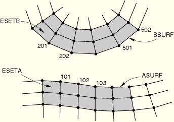
The following input defines finite-sliding contact between the surfaces ASURF and BSURF, shown in Figure 29.2.2–1, with ASURF acting as the slave surface:
*SURFACE, NAME=ASURF
ESETA,
*SURFACE, NAME=BSURF
ESETB,
*CONTACT PAIR, INTERACTION=PAIR1
ASURF, BSURF
*SURFACE INTERACTION, NAME=PAIR1
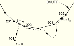
In the example shown in Figure 29.2.2–1, which uses the default finite-sliding, node-to-surface formulation, slave node 101 may come into contact anywhere along the master surface BSURF. While in contact, it is constrained to slide along BSURF, irrespective of the orientation and deformation of this surface. This behavior is possible because ABAQUS/Standard tracks the position of node 101 relative to the master surface BSURF as the bodies deform. Figure 29.2.2–2 shows the possible evolution of the contact between node 101 and its master surface BSURF. Node 101 is in contact with the element face with end nodes 201 and 202 at time ![]() . The load transfer at this time occurs between node 101 and nodes 201 and 202 only. Later on, at time
. The load transfer at this time occurs between node 101 and nodes 201 and 202 only. Later on, at time ![]() , node 101 may find itself in contact with the element face with end nodes 501 and 502. Then the load transfer will occur between node 101 and nodes 501 and 502.
, node 101 may find itself in contact with the element face with end nodes 501 and 502. Then the load transfer will occur between node 101 and nodes 501 and 502.
The finite-sliding, node-to-surface contact formulation requires that master surfaces have continuous surface normals at all points. Convergence problems can result if master surfaces that do not have continuous surface normals are used in finite-sliding, node-to-surface contact analyses; slave nodes tend to get “stuck” at points where the master surface normals are discontinuous. ABAQUS/Standard automatically smooths the surface normals of element-based master surfaces (see “Smoothing deformable master surfaces and rigid surfaces defined with rigid elements” below) used in finite-sliding, node-to-surface contact simulations, including those modeled with slide lines. You are expected to create smooth analytical rigid surfaces (see “Defining analytical rigid surfaces,” Section 2.3.4). No such smoothing of master surface normals is needed with the finite-sliding, surface-to-surface formulation.
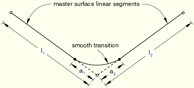
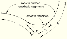
For finite-sliding, node-to-surface contact simulations with planar or axisymmetric deformable master surfaces, ABAQUS/Standard will smooth any discontinuous transitions between two first-order element faces with parabolic curves. Discontinuous transitions between two second-order element faces are smoothed with cubic curves connecting two points located on the element's faces. This smoothing is shown in Figure 29.2.2–3 for first-order elements (linear segments) and in Figure 29.2.2–4 for second-order elements (parabolic segments). For finite-sliding, node-to-surface simulations with three-dimensional deformable master surfaces and rigid master surfaces using rigid elements, ABAQUS/Standard will smooth any discontinuous surface normal transitions between the master surface facets.
You can control the degree of smoothing of the master surface in node-to-surface contact simulations or in analyses using slide lines and contact elements by specifying a fraction f. The default value of f is 0.2.
For planar or axisymmetric deformable master surfaces, ![]() , where
, where ![]() and
and ![]() are the lengths of the element facets that join at the surface node and
are the lengths of the element facets that join at the surface node and ![]() (see Figure 29.2.2–3 and Figure 29.2.2–4).
(see Figure 29.2.2–3 and Figure 29.2.2–4).
For three-dimensional deformable master surfaces and rigid master surfaces using rigid elements, f is defined as a fraction of the dimension of a facet as shown in Figure 29.2.2–5.
The normal vector of a point within the region bounded by the dashed lines is computed to be normal to the facet. Outside this region it is smoothed with respect to the adjacent facets, using a generalization of the two-dimensional approach shown in Figure 29.2.2–3 and Figure 29.2.2–4.| Input File Usage: | Use the following option for node-to-surface contact simulations: |
*CONTACT PAIR, INTERACTION=interaction_property_name, SMOOTH=f Use the following option when using slide lines and contact elements: *SLIDE LINE, ELSET=name, SMOOTH=f |
| ABAQUS/CAE Usage: | Interaction module: Interaction |
When a two-dimensional or axisymmetric deformable master surface ends at a symmetry plane and node-to-surface discretization is used, ABAQUS/Standard will smooth and calculate the proper surface normals and tangent planes of the end segment if the boundary condition at the symmetry end is specified with the symmetry “type” boundary XSYMM or YSYMM. This smoothing procedure is accomplished by reflecting the end segment about the symmetry plane and constructing either a parabolic or a cubic segment between the end segment and the reflected segment. Thus, the contact surface may differ from the faceted element geometry near the end. ABAQUS/Standard will automatically adjust the surface normal and tangent planes at ![]() of an axisymmetric master surface regardless of whether a symmetry boundary condition is defined.
of an axisymmetric master surface regardless of whether a symmetry boundary condition is defined.
To model a master surface with corners in two dimensions (fold lines in three dimensions), break the surface into multiple surfaces. This technique prevents ABAQUS/Standard from smoothing out the corners or fold lines and allows ABAQUS/Standard to introduce constraints associated with each surface if a slave node is in contact with an interior corner or fold in the master surface.
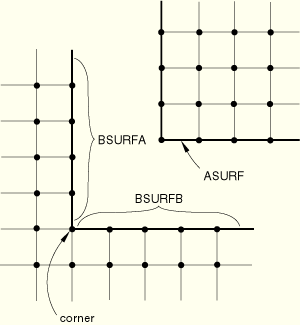
To accurately model the master surface with a corner shown in Figure 29.2.2–6, you must define two contact pairs: the first contact pair has ASURF as the slave surface and BSURFA as the master surface; the second contact pair has ASURF as the slave surface and BSURFB as the master surface.
Finite-sliding simulations usually include nonlinear geometric effects because such simulations generally involve large deformations and large rotations. However, it is also possible to use the finite-sliding tracking approach in a geometrically linear analysis (see “Geometric nonlinearity” in “General and linear perturbation procedures,” Section 6.1.2). The load transfer paths between the surfaces and the contact direction are updated in finite-sliding, geometrically linear analyses. This capability is useful for analyzing finite sliding between two stiff bodies that do not undergo large rotations.
Normal contact constraints due to node-to-surface discretization produce unsymmetric terms in the system of equations when three-dimensional faceted surfaces come in contact. These terms have a strong effect on the convergence rate in regions on the master surfaces with large differences in surface normals between facets.
Normal contact constraints due to surface-to-surface discretization produce unsymmetric terms in both two- and three-dimensional cases. These terms have a strong effect on the convergence rate in regions where the master and slave surfaces are not parallel to each other.
In both cases you should use the unsymmetric solution scheme for the step to improve the convergence rate of the simulation (see “Matrix storage and solution scheme in ABAQUS/Standard” in “Procedures: overview,” Section 6.1.1).
Contact simulations that involve strong frictional effects can also produce unsymmetric terms. See “Unsymmetric terms in the system of equations” in “Frictional behavior,” Section 30.1.5, for details.
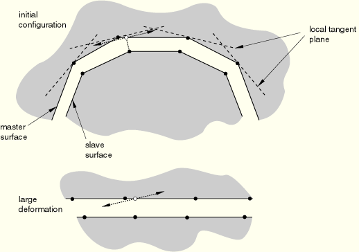
For a large class of contact problems the general tracking of the finite-sliding approach is unnecessary, even though geometric nonlinearity may need to be considered. ABAQUS/Standard provides a small-sliding tracking approach for such problems. For geometrically nonlinear analyses this formulation assumes that the surfaces may undergo arbitrarily large rotations but that a slave node will interact with the same local area of the master surface throughout the analysis. For geometrically linear analyses the small-sliding approach reduces to an infinitesimal-sliding and rotation approach, in which it is assumed that both the relative motion of the surfaces and the absolute motion of the contacting bodies are small.
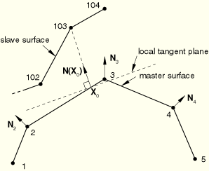
In a small-sliding analysis every slave node interacts with its own local tangent plane on the master surface (see Figure 29.2.2–7). The slave node is constrained not to penetrate this local tangent plane. Each local tangent plane, which is a line in two dimensions, is defined by an anchor point, ![]() , on the master surface and an orientation vector at the anchor point (see Figure 29.2.2–7). The small-sliding, node-to-surface formulation uses a continuously varying surface normal on the master surface to determine the anchor point and the tangent plane.
, on the master surface and an orientation vector at the anchor point (see Figure 29.2.2–7). The small-sliding, node-to-surface formulation uses a continuously varying surface normal on the master surface to determine the anchor point and the tangent plane.
Figure 29.2.2–7 Definition of the anchor point and local tangent plane used by the small-sliding, node-to-surface formulation for node 103.
Having a local tangent plane for each slave node means that for the small-sliding tracking approach ABAQUS/Standard does not have to monitor slave nodes for possible contact along the entire master surface. Therefore, small-sliding contact is less expensive computationally than finite-sliding contact. The cost savings are most dramatic in three-dimensional contact problems.
For node-to-surface contact ABAQUS/Standard chooses the anchor point of a slave node's local tangent plane such that the vector from the anchor point to the slave node coincides with a smoothly varying normal vector on the master surface. The anchor point is chosen before the analysis starts using the initial configuration of the model.
The algorithm requires that the master surface have a smoothly varying normal vector ![]() , where
, where ![]() is any point on the master surface. The first step in defining
is any point on the master surface. The first step in defining ![]() is to construct the unit normal vectors at each node of the master surface. ABAQUS/Standard forms these nodal normals by averaging the normals of the element faces making up the master surface; only the element faces in the surface definition will contribute to the nodal normals and, thus, to
is to construct the unit normal vectors at each node of the master surface. ABAQUS/Standard forms these nodal normals by averaging the normals of the element faces making up the master surface; only the element faces in the surface definition will contribute to the nodal normals and, thus, to ![]() . ABAQUS/Standard uses the initial nodal coordinates to compute these normals.
. ABAQUS/Standard uses the initial nodal coordinates to compute these normals.
Figure 29.2.2–7 shows the nodal unit normals for a master surface, the anchor point ![]() , and the local tangent plane associated with slave node 103. ABAQUS/Standard uses the nodal unit normals
, and the local tangent plane associated with slave node 103. ABAQUS/Standard uses the nodal unit normals ![]() and
and ![]() , along with the shape functions of the element containing the two nodes, to construct
, along with the shape functions of the element containing the two nodes, to construct ![]() on the 2–3 element face. ABAQUS/Standard chooses the anchor point
on the 2–3 element face. ABAQUS/Standard chooses the anchor point ![]() of the local tangent plane for node 103 so that
of the local tangent plane for node 103 so that ![]() passes through node 103.
passes through node 103. ![]() is the contact direction for slave node 103 and defines the orientation of the local tangent plane. In this example, as in many cases, the local tangent plane is only an approximation of the actual mesh geometry.
is the contact direction for slave node 103 and defines the orientation of the local tangent plane. In this example, as in many cases, the local tangent plane is only an approximation of the actual mesh geometry.
Sometimes the default smoothed master surface normal and the local tangent plane that ABAQUS/Standard calculates are not suitable for the desired analysis. The most common situation where unsuitable surface normals are calculated occurs when a curved master surface ends at a symmetry plane and the boundary conditions have been specified in direct format rather than in symmetry “type” format (XSYMM, YSYMM, or ZSYMM—see “Boundary conditions,” Section 27.3.1). In this case the correct normals should be in the symmetry plane; however, because the surface facets that abut the symmetry plane usually form an angle with the plane, the normal will project away from the symmetry plane. The effect of this behavior can be that a slave node does not have a normal from the master surface pass through it (the slave node is said not to “intersect” the master surface). No contact constraints will be enforced for such slave nodes.
A message is printed in the data (.dat) file whenever a slave node does not intersect its master surface. By specifying the proper symmetry “type” boundary condition, ABAQUS/Standard will calculate the correct normal and local tangent planes along the symmetry planes of the master surface.
If the smoothed normals of the master surface and the local tangent planes calculated by ABAQUS/Standard are unsuitable and it is not feasible to apply symmetry “type” boundary conditions, several other methods are available for modifying the smoothed normals. One method is to add or remove some of the element faces making up the master surface. However, this method can influence only the surface normals near the perimeter of the master surface.
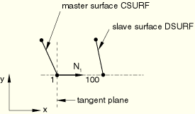
The other method is to modify the nodal normals on the master surface by defining user-specified normals (see “Normal definitions at nodes,” Section 2.1.4). This method is especially useful in providing a more accurate representation of the surface geometry. Figure 29.2.2–8 shows two concentric cylinders that contact each other; the inner cylinder is chosen as the master surface CSURF.
Figure 29.2.2–8 Master surface normal at node 1 in a small-sliding model of concentric cylinders. With the default ![]() slave node 100 will never contact CSURF.
slave node 100 will never contact CSURF.
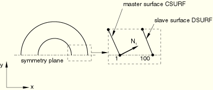
If a half-symmetry model is used, the default master surface normal at the symmetry plane will cause problems. As shown in Figure 29.2.2–8, the nodal normal ![]() does not point along the symmetry plane, which means that slave node 100 will never intersect the master surface. In a small-sliding problem if a slave node fails to intersect the master surface at the start of the analysis, it will be free to penetrate the master surface because no local tangent plane will be formed. ABAQUS/Standard provides the initial contact status—open, overclosed, or “no intersection”—in the data file for every slave node in the model (see “Checking contact conditions in the data file” below). Use this information to confirm that the necessary tangent planes for a model have been found.
does not point along the symmetry plane, which means that slave node 100 will never intersect the master surface. In a small-sliding problem if a slave node fails to intersect the master surface at the start of the analysis, it will be free to penetrate the master surface because no local tangent plane will be formed. ABAQUS/Standard provides the initial contact status—open, overclosed, or “no intersection”—in the data file for every slave node in the model (see “Checking contact conditions in the data file” below). Use this information to confirm that the necessary tangent planes for a model have been found.
In situations such as that shown in Figure 29.2.2–8, define a YSYMM “type” boundary condition at node 1 to specify the symmetry plane. The master normal at the node on the symmetry plane will be modified to lie along the symmetry plane, allowing slave node 100 to see the master surface CSURF.
In situations where a symmetry “type” boundary condition cannot be specified, define a user-specified normal (1.00E+00, 0.00E+00, 0.00E+00) at node 1 on the master surface CSURF to correct the problem. This method will also allow slave node 100 to see the master surface.
The modification to CSURF's normal at node 1, which makes CSURF a better approximation of the actual surface, is shown in Figure 29.2.2–9.
The algorithm to establish the anchor point location for surface-to-surface contact is more complex in most respects than the algorithm for node-to-surface contact. For this approach the anchor point is the center of the zone on the master surface that is closest to the slave surface zone around the slave node. Therefore, it does not need to make use of smoothed master surface nodal normals. The anchor point location typically does not depend significantly on whether node-to-surface or surface-to-surface discretization is used. Since the constraints are based on surface-to-surface discretization it is not necessary that the constraint associated with a node on a symmetry plane is parallel to the symmetry plane. Hence, there is usually no need to specify specific normal directions. As in the case of node-to-surface contact, the contact direction points from the anchor point to the slave node, and the tangent plane is normal to this direction.
The local tangent plane is by definition orthogonal to the contact direction. You can override the default contact direction to specify a direction with a spatially varying clearance or overclosure definition (see “Specifying the surface normal for the contact calculations” in “Adjusting initial surface positions and specifying initial clearances in ABAQUS/Standard contact pairs,” Section 29.2.5).
Once the contact direction is defined, the orientation of the local tangent plane with respect to the master surface facet remains fixed. Because small-sliding contact considers nonlinear geometric effects, ABAQUS/Standard continuously updates the orientation of the local tangent plane to account for the rotation and, assuming that the master surface is deformable, the deformation of the master surface. The position of the anchor point relative to the surrounding nodes on the master surface facet does not change as the master surface deforms.
In a small-sliding analysis the slave node can transfer load only to a limited number of nodes on the master surface. These nodes on the master surface are chosen based on their proximity to the slave node's anchor point. The magnitude of load transferred to each master surface node is weighted by its proximity to the slave node when the slave node contacts the local tangent plane. For example, in Figure 29.2.2–7 node 103 transmits load to both nodes 2 and 3 on the master surface if node-to-surface discretization is used (if surface-to-surface discretization is used, load may be transmitted to additional nearby master nodes). Thus, if node 103 contacts the local tangent plane, a larger share of the force would be transmitted to the master surface node, 2 or 3, closer to the slave node.
When the anchor point ![]() corresponds to a node on the master surface, as is the case with slave node 104 and master surface node 3 in Figure 29.2.2–7, the transmitted load for node-to-surface contact is shared by the node at
corresponds to a node on the master surface, as is the case with slave node 104 and master surface node 3 in Figure 29.2.2–7, the transmitted load for node-to-surface contact is shared by the node at ![]() and all of the master surface nodes that share an adjacent surface facet with that node (additional master nodes may take part in the load transfer for surface-to-surface contact). In Figure 29.2.2–7 the three master surface nodes sharing the force transmitted by slave node 104 are nodes 2, 3, and 4.
and all of the master surface nodes that share an adjacent surface facet with that node (additional master nodes may take part in the load transfer for surface-to-surface contact). In Figure 29.2.2–7 the three master surface nodes sharing the force transmitted by slave node 104 are nodes 2, 3, and 4.
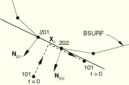
As a slave node slides along its local tangent plane, ABAQUS/Standard updates the distribution of load transferred by a given slave node to its associated master surface nodes. However, no additional master surface nodes are ever added to the original list of nodes associated with a given slave node. The slave node will continue to transmit load to the original list of master surface nodes, regardless of the distance slid by the slave node along its contact plane. Figure 29.2.2–10 shows the potential problem that arises if small sliding is used but the relative tangential motion of the surfaces is not “small.” It shows the possible evolution of contact between slave node 101 in Figure 29.2.2–1 and its master surface BSURF. Using the unit normal vectors ![]() and
and ![]() , the anchor point
, the anchor point ![]() is found for slave node 101; for the purposes of this example, assume that it lies at the midpoint of the 201–202 face. With this location of
is found for slave node 101; for the purposes of this example, assume that it lies at the midpoint of the 201–202 face. With this location of ![]() the local tangent plane for node 101 is parallel with the 201–202 face. The load transfer always occurs between node 101 and nodes 201 and 202, no matter how far node 101 slides along the local tangent plane. Therefore, if node 101 moves as shown in Figure 29.2.2–10, it will continue to transmit load to nodes 201 and 202 when, in fact, it really slid off the mesh forming the master surface BSURF.
the local tangent plane for node 101 is parallel with the 201–202 face. The load transfer always occurs between node 101 and nodes 201 and 202, no matter how far node 101 slides along the local tangent plane. Therefore, if node 101 moves as shown in Figure 29.2.2–10, it will continue to transmit load to nodes 201 and 202 when, in fact, it really slid off the mesh forming the master surface BSURF.
A contact pair in a small-sliding contact simulation should not grossly violate any of the assumptions or limitations outlined above. Adhere to the following guidelines:
Slave nodes should slide less than an element length from their corresponding anchor point and still be contacting their local tangent plane. If the master surface is highly curved, the slave nodes should slide only a fraction of an element length. The accumulated slip at a slave node (CSLIP) can provide a good estimate of how far a slave node has moved.
The local tangent planes formed by ABAQUS/Standard should be a good approximation of the mesh geometry; if necessary, define a user-specified normal (“Normal definitions at nodes,” Section 2.1.4) to improve the smoothly varying master surface normal, ![]() .
.
The rotation and deformation of the master surface should not cause the local tangent planes to become a poor representation of the master surface during the course of the analysis.
The basic guidelines given in “Defining contact pairs in ABAQUS/Standard,” Section 29.2.1, should still be followed in a small-sliding simulation—the slave surface should be the more refined surface or the surface on the more deformable body. However, in a small-sliding simulation more thought must be given when defining the master surface. With small-sliding contact each slave node views the master surface as a flat surface, which can be significantly different than the true shape of the surface, even in the local region near the anchor point. In some cases the local tangent planes provide a good local approximation to the master surface in the initial configuration, but deformation and rotation of the master surface can reorient the local tangent planes such that they become a poor representation of the master surface. Figure 29.2.2–11 shows an example where distortion of the master surface results in such a situation. This problem can be minimized to some extent by using a more refined mesh on the master surface, thus providing more element faces to control the motion of the tangent planes. Excessive mesh refinement should not be necessary since only small sliding should occur.
As was mentioned before, the small-sliding tracking approach reduces to an infinitesimal-sliding tracking approach for geometrically linear analyses. Infinitesimal sliding assumes that both the relative motions of the surfaces and the absolute motions of the model remain small. The orientations of the local tangent planes are not updated, and the load transfer paths and the weightings assigned to each master surface node remain constant during an infinitesimal-sliding simulation.
As in the case of small sliding, you can choose between node-to-surface and surface-to-surface discretizations with the infinitesimal-sliding tracking approach. The same user interface applies, and the default is node-to-surface discretization.
When you request contact constraint information from the analysis input file processor (see “Controlling the amount of analysis input file processor information written to the data file” in “Output,” Section 4.1.1), ABAQUS/Standard provides a table for each contact pair in the data (.dat) file listing the elements and nodes involved in contact. By default, no contact constraint output to the data file is provided.
| Input File Usage: | *PREPRINT, CONTACT=YES |
| ABAQUS/CAE Usage: | Job module: job editor: General: Preprocessor Printout: Print contact constraint data |
In a small-sliding or infinitesimal-sliding simulation, the output table shows the master nodes associated with each slave node so that you can check them. Each row of the table lists a slave node and the master nodes to which the slave node transfers load when in contact with the master surface. The number of nodes in the table indicates whether or not the anchor point for a slave node lies on an element face or at a node.
For example, in the output shown below for a two-dimensional model, slave node 2 has an anchor point at master surface node 101 because it interacts with three master surface nodes. Slave node 1 has an anchor point between nodes 100 and 101. This table also provides a list of slave nodes that did not find an intersection with the master surface. This is important because these nodes can penetrate the master surface since they have no local tangent plane.
The contact element number associated with each slave node is also given in this table. ABAQUS/Standard generates this number automatically. Because the element is not user-defined and does not appear in the input file, it can be difficult to locate it if an error or warning message refers to the contact element number. This table provides the information specifying the location of this internally generated contact element in the model.
SMALL SLIDING  NON-RIGID  AX ELEMENT(S)
        INTERNALLY GENERATED FOR SLAVE BLANK AND MASTER SPHERE
         WITH SURFACE INTERACTION INF1

    ELEMENT  SLAVE   MASTER
    NUMBER   NODE(S) NODE(S)

       46       1     101     100
       47       2     102     101     100
       50       9          NO INTERSECTION
 ***WARNING: 1 SLAVE NODES FOUND NO INTERSECTION WITH A MASTER
SURFACEIn a finite-sliding simulation a similar table is given for every contact pair providing the internally generated contact element number for every facet or node on the slave surface. Because the slave nodes can interact with any portion of the master surface, ABAQUS/Standard gives no information about which slave nodes interact with which portions of the master surface.
All of the contact formulations except the finite-sliding, node-to-surface formulation account for initial shell and membrane thicknesses for element-based surfaces by default. The finite-sliding, node-to-surface formulation will not account for surface thickness. Node-based surfaces have no thickness, regardless of which element types are connected to the surface nodes. Accounting for element thicknesses in contact calculations is generally desirable, but you can avoid having thickness considered if it is not desired.
| Input File Usage: | *CONTACT PAIR, NO THICKNESS |
| ABAQUS/CAE Usage: | Interaction module: interaction editor: Sliding formulation: Small sliding or Finite sliding, Constraint enforcement method: Surface to surface or Node to surface, toggle on Exclude shell/membrane element thickness |
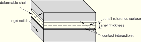
Consider the case of a shell pinched between two rigid surfaces, as shown in Figure 29.2.2–12. In this example contact pairs using the small-sliding, node-to-surface formulation are defined between the top surface of the shell and the top rigid surface and between the bottom surface of the shell and the bottom rigid surface. Although the shell surfaces are defined at the shell reference location, the contact interactions account for the thickness of the shell and are offset from the reference surface. The penalty constraint enforcement method (see “Contact pressure-overclosure relationships,” Section 30.1.2) is used to avoid overconstraining slave nodes. The following input is used:
*SURFACE, NAME=TOP_RIG_SURF
TOP_RIG_ELS,
*SURFACE, NAME=SHELL_TOP_SURF
SHELL_ELS,SPOS
*SURFACE, NAME=SHELL_BOT_SURF
SHELL_ELS,SNEG
*SURFACE, NAME=BOT_RIG_SURF
BOT_RIG_ELS,
*CONTACT PAIR, INTERACTION=INTER_AL, SMALL SLIDING
SHELL_TOP_SURF, TOP_RIG_SURF
SHELL_BOT_SURF, BOT_RIG_SURF
*SURFACE INTERACTION, NAME=INTER_AL
*SURFACE BEHAVIOR, PENALTY
ABAQUS/Standard calculates the initial orientation of the two slip directions by default. However, if the default slip directions are not convenient to prescribe an anisotropic friction model or to view contact output, you can define the slip directions. These slip directions will rotate with the contact pair in a geometrically nonlinear analysis.
By default, ABAQUS/Standard determines the initial orientation of the two slip directions, ![]() and
and ![]() , using the following conventions.
, using the following conventions.
Finite sliding: The default initial orientations of the two slip directions are calculated at each contact point on the slave surface based on the negative normal at that point, using the standard convention for calculating surface tangents (see “Conventions,” Section 1.2.2). For the node-based slave surface the initial slip directions coincide with the global x- and y-axes with the normal being along the z-axis. For node-to-surface discretization, the negative normal is then aligned with the master surface normal, changing the slip directions accordingly.
Small sliding: The default initial orientations of the two slip directions are calculated at each point on the master surface based on the master surface normal, using the standard convention for calculating surface tangents.
Exceptions to these conventions arise when slave surfaces are generated from three-dimensional beam, truss, or pipe elements and used in finite-sliding contact; when surfaces are created on generalized axisymmetric elements; or for deformable versus analytical rigid surface contact with the finite-sliding, node-to-surface formulation.
For slave surfaces attached to three-dimensional beam-type elements and used in finite-sliding contact, the first and second slip directions are always defined along the length of the beam and transverse to the beam, respectively.
For surfaces on generalized axisymmetric bodies, the first slip direction at any point on the surface is always tangent to the surface in the local r–z plane. The second slip direction is orthogonal to this plane in the local circumferential direction.
For deformable versus analytical rigid surface contact with the finite-sliding, node-to-surface formulation, the first slip direction is tangential to the cross-section used to generate the analytical rigid surface, and the second slip direction is orthogonal to the plane of the cross-section in which the contact occurs.
Alternatively, you can define the slip directions by associating an orientation definition (see “Orientations,” Section 2.2.5) with a contact pair surface, with the exception of finite-sliding contact between a deformable slave surface and an analytical rigid surface. You can assign an orientation only to one surface of a contact pair. The surface on which an orientation can be defined is the same surface on which the default orientation would be calculated (see the conventions given previously). For example, an orientation can be defined only on the slave surface in deformable versus deformable finite-sliding contact. If a second orientation is also given, an error message is issued. An orientation that is defined on a slave surface of a contact pair that is generated from three-dimensional truss-type elements or from a list of nodes without rotational degree of freedoms will not be rotated if the slave surface undergoes finite motion. In this case a warning message is issued during input processing.
| Input File Usage: | *CONTACT PAIR, INTERACTION=interaction_property_name slave surface name, master surface name, orientation for slave surface slave surface name, master surface name, , orientation for master surface |
| ABAQUS/CAE Usage: | You cannot define alternative slip directions for contact pairs in ABAQUS/CAE. |
For geometrically nonlinear analyses the tangential slip directions of a contact pair rotate with the surface on which these directions were initially calculated or redefined using an orientation definition as described above. These rotated tangential slip directions are further rotated to ensure that the normal vector, computed using the cross product of the rotated tangential slip directions, corresponds to the normal vector on the master surface when the slave node comes into contact.