Products: ABAQUS/Explicit ABAQUS/CAE
The contact formulation for the contact pair algorithm in ABAQUS/Explicit includes:
the constraint enforcement method (kinematic or penalty);
the contact surface weighting (balanced or pure master-slave); and
the sliding formulation (finite, small, or infinitesimal).
By default, all contact pairs in an ABAQUS/Explicit simulation use a kinematic predictor/corrector contact algorithm to strictly enforce contact constraints (for example, no penetrations are allowed). Alternatively you can choose a penalty contact algorithm, which has a weaker enforcement of contact constraints but allows for treatment of more general types of contact. Both methods conserve momentum between the contacting bodies.
A summary of the default kinematic algorithm that ABAQUS/Explicit uses to enforce contact with the contact pair algorithm is presented below. It is a predictor/corrector algorithm and, therefore, has no influence on the stable time increment. It is easier to describe the algorithm by first considering a pure master-slave contact pair.
In this case in each increment of the analysis ABAQUS/Explicit first advances the kinematic state of the model into a predicted configuration without considering the contact conditions. ABAQUS/Explicit then determines which slave nodes in the predicted configuration penetrate the master surfaces. The depth of each slave node's penetration, the mass associated with it, and the time increment are used to calculate the resisting force required to oppose penetration. For hard contact, this is the force which, had it been applied during the increment, would have caused the slave node to exactly contact the master surface. The next step depends on the type of master surface used.
When the master surface is formed by element faces, the resisting forces of all the slave nodes are distributed to the nodes on the master surface. The mass of each contacting slave node is also distributed to the master surface nodes and added to their mass to determine the total inertial mass of the contacting interfaces. ABAQUS/Explicit uses these distributed forces and masses to calculate an acceleration correction for the master surface nodes. Acceleration corrections for the slave nodes are then determined using the predicted penetration for each node, the time increment, and the acceleration corrections for the master surface nodes. ABAQUS/Explicit uses these acceleration corrections to obtain a corrected configuration in which the contact constraints are enforced.
In the case of an analytical rigid master surface, the resisting forces of all slave nodes are applied as generalized forces on the associated rigid body. The mass of each contacting slave node is added to the rigid body to determine the total inertial mass of the contacting interfaces. The generalized forces and added masses are used to calculate an acceleration correction for the analytical rigid master surface. Acceleration corrections for the slave nodes are then determined by the corrected motion of the master surface.
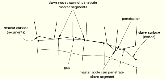
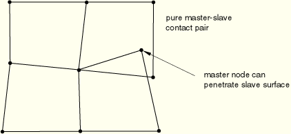
When using hard kinematic contact, it is still possible with the pure master-slave algorithm for the master surface to penetrate the slave surface in the corrected configuration (see Figure 29.4.4–1).
Using a sufficiently refined mesh on the slave surface will minimize such penetrations. Softened kinematic contact will allow penetrations since corrections are made to satisfy the pressure-overclosure relationship at the slave-nodes, not the condition of zero penetration.The kinematic contact algorithm for a balanced master-slave contact pair applies acceleration corrections that are linear combinations of pure master-slave corrections calculated in exactly the same manner as outlined above. One set of corrections is calculated considering one surface as the master surface, and the other corrections are calculated considering that same surface as the slave surface. ABAQUS/Explicit then applies a weighted average of the two values. The exact weighting for each correction depends on the weighting factor specified for the contact pair (see “Contact surface weighting” below). The default for balanced master-slave contact is to weight each correction equally.
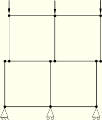
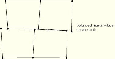
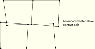
Hard kinematic contact will minimize the penetration of the surfaces. However, after the initial weighted correction is applied, it is possible to still have some penetration of the surfaces. Therefore, ABAQUS/Explicit uses a second contact correction to resolve any remaining overclosure in a balanced master-slave contact pair that uses hard kinematic contact (a second contact correction is not conducted for softened kinematic contact). Both master-slave assignment combinations are again considered, but weighting factors are not used when combining the contributions to form the second applied acceleration correction. It is possible that small gaps between the contacting surfaces will be created during the second correction if there was some residual penetration after the first correction: the magnitude of the gaps after the second correction will generally be much smaller than the penetration after the first correction. The effect of the second correction is illustrated in Figure 29.4.4–2 to Figure 29.4.4–5.
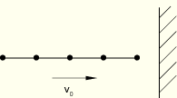
The kinematic contact algorithm strictly enforces contact constraints and conserves momentum. To achieve these qualities with a discretized model, some energy is absorbed upon impact. For example, consider a linear elastic beam modeled with several elements that impacts a rigid wall as shown in Figure 29.4.4–6. The kinetic energy of the leading node is absorbed by the contact algorithm upon impact. A stress wave passes through the truss, and the truss eventually rebounds from the wall. The kinetic energy after the rebound is smaller than before the impact because of the contact node's energy loss upon impact. As the mesh is refined, this energy loss is reduced because the mass and kinetic energy of the leading node of the truss become less significant.
Contact forces can also exert negative external work upon impact since contact forces act over the entire increment in which impact occurs, including the fraction of the increment prior to impact. The opposing contact forces, which are equal in magnitude, act over different distances, thereby exerting a nonzero net work. The net external work of these forces is negative, and the absolute value of the net external work does not exceed the contact node's kinetic energy loss upon impact. These energies are insignificant in most models but can be significant in high-speed impacts, where high mesh refinement near the contact interface is recommended.
The penalty contact algorithm results in less stringent enforcement of contact constraints than the kinematic contact algorithm, but the penalty algorithm allows for treatment of more general types of contact (for example, contact between two rigid bodies). When the penalty method is chosen for enforcing contact constraints in the normal direction, it is also used to enforce sticking friction (see “Frictional behavior,” Section 30.1.5). Since the penalty algorithm introduces additional stiffness behavior into a model, this stiffness can influence the stable time increment. ABAQUS/Explicit automatically accounts for the effect of the penalty stiffnesses in the automatic time incrementation, although this effect is usually small, as discussed below.
| Input File Usage: | Use the following option to select the penalty contact algorithm: |
*CONTACT PAIR, MECHANICAL CONSTRAINT=PENALTY surface_1, surface_2 |
| ABAQUS/CAE Usage: | Interaction module: interaction editor: Mechanical constraint formulation: Penalty contact method |
The penalty contact algorithm searches for slave node penetrations in the current configuration. Contact forces that are a function of the penetration distance are applied to the slave nodes to oppose the penetration, while equal and opposite forces act on the master surface at the penetration point. When the master surface is formed by element faces, the master surface contact forces are distributed to the nodes of the master faces being penetrated. In the case of an analytical rigid master surface, the master surface forces are applied as forces and moments on the associated rigid body.
The “spring” stiffness that relates the contact force to the penetration distance is chosen automatically by ABAQUS/Explicit for hard penalty contact, such that the effect on the time increment is minimal yet the allowed penetration is not significant in most analyses. The penetration distance will typically be an order of magnitude greater than the parent elements' elastic deformation normal to the contact interface. In purely elastic problems this penetration can affect the stress solution significantly, as demonstrated in “The Hertz contact problem,” Section 1.1.11 of the ABAQUS Benchmarks Manual. You can specify a factor by which to scale the default penalty stiffnesses. Penalty stiffnesses obtained from a user-defined softened contact relationship are not scaled by this factor. This scaling may affect the automatic time incrementation. Use of a large scale factor is likely to increase the computational time required for an analysis because of the reduction in the time increment that is necessary to maintain numerical stability.
As with the pure master-slave kinematic contact algorithm, there is no resistance to master surface nodes penetrating slave surface faces with the pure master-slave penalty contact algorithm. Using a sufficiently refined mesh on the slave surface will help correct this problem.
| Input File Usage: | Use both of the following options to scale the default penalty stiffnesses: |
*CONTACT PAIR, MECHANICAL CONSTRAINT=PENALTY, CPSET=contact_pair_set_name surface_1, surface_2 *CONTACT CONTROLS, CPSET=contact_pair_set_name, SCALE PENALTY=factor |
| ABAQUS/CAE Usage: | Interaction module: Create Contact Controls: Name: contact_controls_name, ABAQUS/Explicit contact controls: Penalty stiffness scaling factor: factor |
Interaction editor: Mechanical constraint formulation: Penalty contact method, Contact controls: contact_controls_name |
The penalty contact algorithm for a balanced master-slave contact pair computes contact forces that are linear combinations of pure master-slave forces calculated in the manner outlined above. One set of forces is calculated considering one surface as the master surface, and the other forces are calculated considering that same surface as the slave surface. ABAQUS/Explicit then applies a weighted average of the two values. The weighting used with each set of forces depends on the weighting factor specified for the contact pair (see “Contact surface weighting” below). The default for balanced master-slave contact is to weight each of the two sets of forces equally.
The penalty contact algorithm can model some types of contact that the kinematic contact algorithm cannot. Element-based rigid surfaces are not restricted to acting only as master surfaces within the penalty algorithm as they are within the kinematic algorithm. Thus, the penalty method allows modeling of contact between rigid surfaces, except when both surfaces are analytical rigid surfaces or when both surfaces are node-based.
The penalty contact algorithm must be used for all contact pairs involving a rigid body if a linear constraint equation, multi-point constraint, surface-based tie constraint, or connector element is defined for a node on the rigid body. For all other cases, ABAQUS/Explicit enforces equations, multi-point constraints, tie constraints, embedded element constraints, and kinematic constraints (defined using connector elements) independently of contact constraints; therefore, if a degree of freedom participates in a linear constraint equation, multi-point constraint, tie constraint, embedded element constraint, or kinematic constraint in addition to a contact constraint, the contact constraint will usually override these constraints (see the discussion in “Conflicts with multi-point constraints” in “Common difficulties associated with contact modeling using the contact pair algorithm in ABAQUS/Explicit,” Section 29.4.6). Hence, the penalty contact algorithm is recommended if these constraints need to be strictly enforced.
Impact is plastic when the default hard, kinematic contact algorithm is used; and the kinetic energy of the contacting nodes is lost. This loss in energy is insignificant for a refined mesh but can be significant with a coarse mesh. Penalty contact and softened kinematic contact introduce numerical softening to the contact enforcement analogous to adding elastic springs to the contact interface, which means that these algorithms do not dissipate energy upon impact (the energy stored in the springs is recoverable). This distinction between the algorithms is particularly apparent if a point mass with no force acting upon it impacts a fixed rigid wall: with penalty contact and softened kinematic contact the point mass will bounce away, but with hard kinematic contact the point mass will stick to the wall.
A further difference between kinematic and penalty contact is that the critical time increment is unaffected by kinematic contact but can be affected by penalty contact. For hard penalty contact, default penalty stiffnesses are chosen such that the stable time increments of the deformable parent elements of contact surface facets are effectively reduced by approximately 4% for increments in which contact forces are being transmitted; default penalty stiffnesses of node-based surface nodes require a 1% decrease in the element-by-element time increment to ensure numerical stability. Penalty stiffnesses between rigid bodies are chosen by default to have no effect on the stable time increment. If the default penalty stiffnesses are overridden by a penalty scale factor or softened contact behavior (see “Contact pressure-overclosure relationships,” Section 30.1.2), the time increment is modified based on the maximum stiffness active in the contact interface. Increasing the penalty stiffnesses may decrease the stable time increment significantly (see Table 29.4.4–1). If the overall stable time increment is not controlled by elements on the contact interface, the penalty contact algorithm usually will not affect the time increment.
Table 29.4.4–1 Effect of scale factor on time increment.
| Penalty scale factor | Lower bound to ratio of the time increment with contact divided by the time increment without contact |
|---|---|
| 1.0 | 0.96 |
| 10.0 | 0.34 |
| 100.0 | 0.13 |
| 1000.0 | 0.04 |
| 10000.0 | 0.013 |
Penalty contact and softened kinematic contact cannot be used with the breakable bond model; hard kinematic contact must be used for this model.
Both the pure master-slave and the balanced master-slave contact algorithms are available in ABAQUS/Explicit. By default, ABAQUS/Explicit will decide which algorithm to use for any given contact pair based on the nature of the two surfaces forming the contact pair and whether kinematic or penalty enforcement of contact constraints is used. You can override the defaults in some cases.
ABAQUS/Explicit uses the pure master-slave, kinematic contact algorithm, by default, in the following situations (the first surface in each situation listed is designated the master surface):
when a rigid surface contacts a deformable surface;
when an element-based surface contacts a node-based surface; or
when a surface based on continuum elements contacts a surface based on shell or membrane elements.
when a single surface contacts itself (referred to as self-contact or single-surface contact); or
when two deformable surfaces that are meshed with similar elements (i.e., either both surfaces have shells or membranes or both have continuum elements) contact each other.
when an analytical rigid surface contacts a deformable surface; or
when an analytical rigid surface or an element-based surface contacts a node-based surface.
when a single surface contacts itself (referred to as self-contact or single-surface contact); or
when two element-based surfaces contact each other.
When the kinematic contact method is chosen, you can override the default contact pair weighting only when two separate deformable element-based surfaces are contacting each other, which corresponds to the last situation in each list for kinematic contact given in the previous section.
The following aspects should be considered when deciding whether or not to override the default choice. First, the balanced master-slave contact algorithm requires more computational time, but it is typically more accurate. Second, when the densities differ by orders of magnitude, the less dense body should be a pure slave surface. Contact-induced noise can occur if a surface on a much denser body is at all weighted as a slave surface. Finally, to avoid significant penetration for hard contact, the surface with the finer mesh should not be the master surface in the pure master-slave contact pair.
When the penalty contact method is chosen, you can choose to specify a pure master-slave weighting to reduce computational time. When two originally flat surfaces contact one another, a more uniform penetration distance distribution may result with pure master-slave weighting as compared to balanced master-slave weighting. This can be particularly evident if the mesh densities of the contacting surfaces differ significantly—with balanced weighting the contact penetrations will be smaller near the nodes of the coarsely meshed surface. However, balanced master-slave weighting provides better enforcement of contact constraints in most cases.
You define a weighting factor, f, to specify the master-slave weighting. Set f=1.0 to designate the first surface in the contact pair as the master surface and the second surface as the slave surface. Set f=0.0 to designate the first surface in the contact pair as the slave surface and the second surface as the master surface. Specifying any value of f between 0 and 1.0 invokes the balanced master-slave contact algorithm. When f=0.5, which is the default for balanced master-slave contact pairs, ABAQUS/Explicit weights each set of corrections equally. In contrast, ABAQUS/Standard uses a pure master-slave contact algorithm; the slave surface must always be given first, as in the f=0.0 case above.
| Input File Usage: | *CONTACT PAIR, WEIGHT=f |
| ABAQUS/CAE Usage: | Interaction module: interaction editor: Weighting factor Specify f |
In ABAQUS/Explicit there are three approaches to account for the relative motion of the two surfaces forming a contact pair:
finite sliding, which is the most general and allows any arbitrary motion of the surfaces;
small sliding, which assumes that although two bodies may undergo large motions, there will be relatively little sliding of one surface along the other; or
infinitesimal sliding and rotation, which assumes that both the relative motion of the surfaces and the absolute motion of the contacting bodies are small.
The finite-sliding formulation allows for arbitrary separation, sliding, and rotation of the surfaces. ABAQUS/Explicit uses this formulation by default.
| Input File Usage: | *CONTACT PAIR |
| ABAQUS/CAE Usage: | Interaction module: interaction editor: Sliding formulation: Finite sliding |
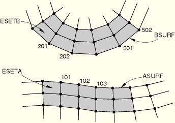
The following input defines finite-sliding contact between the surfaces ASURF and BSURF, shown in Figure 29.4.4–7, with ASURF acting as the slave surface:
*SURFACE,NAME=ASURF
ESETA,
*SURFACE,NAME=BSURF
ESETB,
*CONTACT PAIR,INTERACTION=PAIR1, WEIGHT=0.0
ASURF, BSURF
*SURFACE INTERACTION,NAME=PAIR1
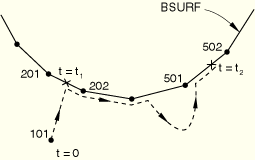
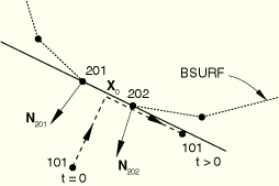
In the example shown in Figure 29.4.4–7 slave node 101 may come into contact anywhere along the master surface BSURF. While in contact, it is constrained to slide along BSURF, irrespective of the orientation and deformation of this surface. This behavior is possible because ABAQUS/Explicit tracks the position of node 101 relative to the master surface BSURF as the bodies deform. Figure 29.4.4–8 shows the possible evolution of the contact between node 101 and its master surface BSURF. Node 101 is in contact with the element face with end nodes 201 and 202 at time ![]() . The load transfer at this time occurs between node 101 and nodes 201 and 202 only. Later on, at time
. The load transfer at this time occurs between node 101 and nodes 201 and 202 only. Later on, at time ![]() , node 101 may find itself in contact with the element face with end nodes 501 and 502. Then the load transfer will occur between node 101 and nodes 501 and 502.
, node 101 may find itself in contact with the element face with end nodes 501 and 502. Then the load transfer will occur between node 101 and nodes 501 and 502.
Finite-sliding simulations usually include nonlinear geometric effects because such simulations generally involve large deformations and large rotations. However, it is also possible to use the finite-sliding formulation in a geometrically linear analysis (see “Geometric nonlinearity” in “General and linear perturbation procedures,” Section 6.1.2). The load transfer paths between the surfaces and the contact direction are updated in finite-sliding, geometrically linear analysis. This capability is useful for analyzing finite sliding between two stiff bodies that do not undergo large rotations.
For a large class of contact problems the general tracking of the finite-sliding formulation is unnecessary, even though geometric nonlinearity must be considered. ABAQUS/Explicit provides a small-sliding contact formulation for such problems. This formulation assumes that the surfaces may undergo arbitrarily large rotations but that a slave node will interact with the same local area of the master surface throughout the analysis. Contact pairs that use the small-sliding formulation must be defined in the first step of the simulation, although they may remain active after the first step.
A large-displacement formulation (the default) should be used for the step in which the small-sliding contact formulation should be used.
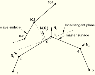
In a small-sliding analysis every slave node interacts with its own local tangent plane on the master surface (see Figure 29.4.4–9). The slave node is constrained not to penetrate this local tangent plane. Each local tangent plane, which is a line in two dimensions, is defined by an anchor point, ![]() , on the master surface and an orientation vector at the anchor point (see Figure 29.4.4–9).
, on the master surface and an orientation vector at the anchor point (see Figure 29.4.4–9).
Having a local tangent plane for each slave node means that for the small-sliding formulation ABAQUS/Explicit does not have to monitor slave nodes for possible contact along the entire master surface. Therefore, small-sliding contact is less expensive computationally than finite-sliding contact. The cost savings are most dramatic in three-dimensional contact problems.
When the balanced master-slave contact algorithm is invoked with the small-sliding formulation, anchor points and tangent planes will be computed for both surfaces.
| Input File Usage: | Use both of the following options: |
*STEP, NLGEOM=YES
…
*CONTACT PAIR, SMALL SLIDING
For example, the following options define small-sliding contact between the two bodies shown in Figure 29.4.4–7: *STEP, NLGEOM=YES … *SURFACE, NAME=ASURF ESETA, *SURFACE, NAME=BSURF ESETB, *CONTACT PAIR, SMALL SLIDING, WEIGHT=0.0 ASURF, BSURF |
| ABAQUS/CAE Usage: | Interaction module: interaction editor: Sliding formulation: Small sliding |
The anchor point and the tangent plane orientation are chosen before the analysis starts using the initial configuration of the model. The anchor point and the tangent plane orientation remain fixed with respect to the master surface facet for all steps in which the contact pair is active. No contact constraints are enforced for slave nodes whose nearest point lies on the free perimeter of the master surface in the original configuration and that do not project onto any master surface facet.
ABAQUS/Explicit chooses the anchor point as the nearest point on the master surface. The orientation of the tangent plane is calculated by default from the normals at the master surface nodes, or you can specify it directly.
Master surface normals: The first step in defining the tangent plane orientation is to construct the unit normal vectors at each node of the master surface. ABAQUS/Explicit forms these nodal normals by averaging the normals of the element faces making up the master surface; only the element faces in the surface definition will contribute to the nodal normals. The tangent plane orientation is then calculated from the master surface nodal normals and the element shape functions at the anchor point.
Figure 29.4.4–9 shows the nodal unit normals for a master surface, the anchor point ![]() , and the local tangent plane associated with slave node 103. ABAQUS/Explicit uses the closest point on the master surface as the anchor point.
, and the local tangent plane associated with slave node 103. ABAQUS/Explicit uses the closest point on the master surface as the anchor point. ![]() is the contact direction for slave node 103 and defines the orientation of the local tangent plane. In this example, as in many cases, the local tangent plane is only an approximation of the actual mesh geometry.
is the contact direction for slave node 103 and defines the orientation of the local tangent plane. In this example, as in many cases, the local tangent plane is only an approximation of the actual mesh geometry.
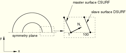
Master surface normals at symmetry planes: Sometimes the master surface normal and the local tangent plane that ABAQUS/Explicit calculates are not suitable for the desired analysis. The most common situation where unsuitable surface normals are calculated occurs when a curved master surface ends at a symmetry plane and the boundary conditions have been specified in direct format rather than in symmetry “type” format (XSYMM, YSYMM, or ZSYMM—see “Boundary conditions,” Section 27.3.1). In this case the correct normals should be in the symmetry plane; however, because the surface facets that abut the symmetry plane usually form an angle with the plane, the normal will project away from the symmetry plane. The effect of this behavior can be that a slave node does not project onto any master surface facet (the slave node is said not to “intersect” the master surface). No contact constraints will be enforced for such slave nodes. However, if symmetry “type” format boundary conditions are specified, contact constraints will be enforced as described below.
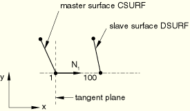
Figure 29.4.4–10 shows two concentric cylinders that contact each other; the inner cylinder is chosen as the master surface CSURF, and a half-symmetry model is used.
Figure 29.4.4–10 Master surface normal at node 1 in a small-sliding model of concentric cylinders. With the default ![]() slave node 100 will never contact CSURF.
slave node 100 will never contact CSURF.
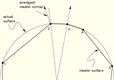
Modifying the local tangent plane orientation: In some cases the contact direction, ![]() , defined from the master surface averaged normals will not define the contact surface accurately. The most common example of this is a circular surface meshed with nonuniform length facets. Figure 29.4.4–12 shows how the averaged master normals will not be oriented correctly in the radial direction.
, defined from the master surface averaged normals will not define the contact surface accurately. The most common example of this is a circular surface meshed with nonuniform length facets. Figure 29.4.4–12 shows how the averaged master normals will not be oriented correctly in the radial direction.
Figure 29.4.4–12 Poorly oriented averaged master surface normals for an irregularly meshed circular surface.
The local tangent plane is always orthogonal to the contact direction. The contact direction is taken as the interpolated normal of the master surface at the anchor point, ![]() , or as the direction specified with a spatially varying clearance definition (see “Specifying initial clearance values precisely” in “Adjusting initial surface positions and specifying initial clearances in ABAQUS/Explicit contact pairs,” Section 29.4.5). Once the contact direction has been defined, the orientation of the local tangent plane with respect to the master surface facet remains fixed. Because the small-sliding formulation considers nonlinear geometric effects, ABAQUS/Explicit continuously updates the orientation of the local tangent plane to account for the rotation of the master surface facet. The position of the anchor point relative to the surrounding nodes on the master surface facet does not change as the master surface deforms.
, or as the direction specified with a spatially varying clearance definition (see “Specifying initial clearance values precisely” in “Adjusting initial surface positions and specifying initial clearances in ABAQUS/Explicit contact pairs,” Section 29.4.5). Once the contact direction has been defined, the orientation of the local tangent plane with respect to the master surface facet remains fixed. Because the small-sliding formulation considers nonlinear geometric effects, ABAQUS/Explicit continuously updates the orientation of the local tangent plane to account for the rotation of the master surface facet. The position of the anchor point relative to the surrounding nodes on the master surface facet does not change as the master surface deforms.
In a small-sliding analysis the slave node will transfer load to the nodes of the master surface facet containing the anchor point, with the magnitude of the load transferred to each node weighted by its proximity to the anchor point. For example, in Figure 29.4.4–9 node 103 transmits load to both nodes 2 and 3 on the master surface. Thus, if node 103 impacts the local tangent plane, a larger share of the force would be transmitted to node 3 because it is closer to the anchor point ![]() .
.
As a slave node slides along its local tangent plane, ABAQUS/Explicit does not update the distribution of load transferred by a given slave node to its associated master surface nodes; the distribution is based solely on the position of the anchor point. This is unlike the small-sliding formulation in ABAQUS/Standard, which does update the load distribution to the master surface nodes as sliding occurs, so that no net moment is associated with the contact forces acting on slave and master nodes per active contact constraint, regardless of the amount of sliding. Some net moment will be associated with the contact forces after sliding has occurred with the small-sliding formulation in ABAQUS/Explicit. This net moment will not be significant if the sliding is truly small compared to element dimensions, but otherwise it can result in non-physical behavior and poor accounting of energy.
Figure 29.4.4–13 shows the potential problem that arises if small sliding is used but the relative tangential motion of the surfaces is not “small.”
It shows the possible evolution of contact between slave node 101 in Figure 29.4.4–7 and its master surface BSURF. Using the unit normal vectorsA contact pair in a small-sliding contact simulation should not grossly violate any of the assumptions or limitations outlined above. Adhere to the following guidelines:
Slave nodes should slide less than an element length from their corresponding anchor point and still be contacting their local tangent plane. If the master surface is highly curved, the slave nodes should slide only a fraction of an element length.
The local tangent planes formed by ABAQUS/Explicit should be a good approximation of the mesh geometry; if necessary, use an initial clearance definition (“Specifying initial clearance values precisely” in “Adjusting initial surface positions and specifying initial clearances in ABAQUS/Explicit contact pairs,” Section 29.4.5) to improve the tangent plane orientation.
The rotation and deformation of the master surface should not cause the local tangent planes to become a poor representation of the master surface during the course of the analysis.
The basic guidelines for pure master-slave contact given previously in this section should still be followed in a small-sliding simulation. However, in a small-sliding simulation more thought must be given to the degree of refinement for the master surface.
The smoothly varying master surface normal ![]() and the local tangent planes that are formed with it are crucial to the success of a small-sliding analysis. As has been mentioned previously, there are several methods that can be used to modify
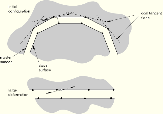
and the local tangent planes that are formed with it are crucial to the success of a small-sliding analysis. As has been mentioned previously, there are several methods that can be used to modify ![]() ; however, they only control the initial configuration of the local tangent planes. The deformation and rotation of the master surface can reorient the local tangent planes such that they become a poor representation of the master surface. Figure 29.4.4–14 shows an example where distortion of the master surface results in such a situation.
; however, they only control the initial configuration of the local tangent planes. The deformation and rotation of the master surface can reorient the local tangent planes such that they become a poor representation of the master surface. Figure 29.4.4–14 shows an example where distortion of the master surface results in such a situation.
The difference between the infinitesimal-sliding and small-sliding formulations is that the infinitesimal-sliding formulation ignores nonlinear geometric effects. To specify the infinitesimal-sliding formulation, you choose the small-sliding contact formulation and a small-displacement formulation for the analysis step.
Infinitesimal sliding assumes that both the relative motions of the surfaces and the absolute motions of the model remain small. The orientations of the local tangent planes are not updated, and the load transfer paths and the weightings assigned to each master surface node remain constant during an infinitesimal-sliding simulation.
| Input File Usage: | Use both of the following options: |
*STEP, NLGEOM=NO … *CONTACT PAIR, SMALL SLIDING |
| ABAQUS/CAE Usage: | Interaction module: interaction editor: Sliding formulation: Small sliding |