Products: ABAQUS/Explicit ABAQUS/CAE
ABAQUS/Explicit provides two algorithms for modeling contact and interaction problems: the general contact algorithm and the contact pair algorithm. See “Contact interaction analysis: overview,” Section 29.1.1, for a comparison of the two algorithms. This section describes how to define contact pairs with surfaces for contact simulations in ABAQUS/Explicit.
Contact pairs in ABAQUS/Explicit:
are part of the history definition of the model and can be created, modified, and removed from step to step (unlike ABAQUS/Standard, where contact pairs are model data);
use sophisticated tracking algorithms to ensure that proper contact conditions are enforced efficiently;
can be used simultaneously with the general contact algorithm (i.e., some interactions can be modeled with contact pairs, while others are modeled with the general contact algorithm);
can be formed using a pair of rigid or deformable surfaces or a single deformable surface;
do not have to use surfaces with matching meshes; and
cannot be formed with one two-dimensional surface and one three-dimensional surface.
The definition of a contact pair interaction in ABAQUS/Explicit consists of specifying:
the contact pair algorithm and the surfaces that interact with one another, as described in this section;
the contact surface properties (“Surface properties for ABAQUS/Explicit contact pairs,” Section 29.4.2);
the mechanical contact property models (“Contact properties for ABAQUS/Explicit contact pairs,” Section 29.4.3);
the contact formulation (“Contact formulation for ABAQUS/Explicit contact pairs,” Section 29.4.4); and
the algorithmic contact controls (“Common difficulties associated with contact modeling using the contact pair algorithm in ABAQUS/Explicit,” Section 29.4.6).
To define a contact pair, you must indicate which pairs of surfaces will interact with each other. The order in which the surfaces are specified is important only when a nondefault weighting factor is specified (see “Contact surface weighting” in “Contact formulation for ABAQUS/Explicit contact pairs,” Section 29.4.4, for details). See “Defining element-based surfaces,” Section 2.3.2; “Defining node-based surfaces,” Section 2.3.3; and “Defining analytical rigid surfaces,” Section 2.3.4, for information on defining surfaces for use in contact pairs.
| Input File Usage: | *CONTACT PAIR surface_1_name, surface_2_name |
| ABAQUS/CAE Usage: | Interaction module: Create Interaction: Surface-to-surface contact (Explicit): select the first surface, click Surface, select the second surface |
Define contact between a single surface and itself by specifying only a single surface or by specifying the same surface twice.
| Input File Usage: | Use either of the following options: |
*CONTACT PAIR surface_1, *CONTACT PAIR surface_1, surface_1 |
| ABAQUS/CAE Usage: | Interaction module: Create Interaction: Self-contact (Explicit): select the surface or Surface-to-surface contact (Explicit): select the surface, click Surface, select the surface again |
The following limitations are enforced for a contact pair with self-contact:
The balanced master-slave contact algorithm will always be used for the contact pair (a nondefault weighting factor cannot be specified for the contact pair).
A contact thickness must be considered for self-contact surfaces on shell or membrane elements (see “Defining element-based surfaces,” Section 2.3.2); i.e., a zero surface thickness (see “Forcing zero surface thickness and offset” in “Surface properties for ABAQUS/Explicit contact pairs,” Section 29.4.2) causes ABAQUS/Explicit to issue an error message. By default, the contact thickness is equal to the current thickness.
The contact thickness for self-contact should not exceed the edge lengths or diagonal lengths of the facets. You can reduce the contact thickness, if necessary; see “Controlling the effects of surface thickness and offset in contact calculations” in “Surface properties for ABAQUS/Explicit contact pairs,” Section 29.4.2.
A specialized finite-sliding tracking algorithm must be used. The use of the small-sliding contact formulation is not supported and causes ABAQUS/Explicit to issue an error message.
Contact will be recognized between any node on a self-contact surface and any other point on the same surface, including either side of shells or membranes (i.e., self-contact on shells and membranes is independent of the face identifier specified in the surface definition).
Removal and addition of contact pairs:
can be used to simulate complicated forming processes where multiple tools need to interact with the workpiece at different stages;
can be used to extend surfaces to prevent one surface from sliding off another;
can result in significant computational savings by eliminating unnecessary contact searches; and
can be used to change the definition of a contact pair.
By default, the contact pairs specified are added to the list of active contact pairs in the model.
Initial penetrations should be avoided for contact pairs introduced after the first step, as large nodal accelerations and severe element distortions can result (see “Adjusting initial surface positions and specifying initial clearances in ABAQUS/Explicit contact pairs,” Section 29.4.5). Redefining a contact pair by deleting it and adding it in the same step can also lead to problems, because the “state” information associated with the slave nodes in contact will be reinitialized. For example, a penalty contact slave node with a penetration past the midsurface of a double-sided master surface would be allowed to pass through the master surface if the contact state were reinitialized.
| Input File Usage: | *CONTACT PAIR, OP=ADD |
| ABAQUS/CAE Usage: | Interaction module: Create Interaction |
Removal of contact pairs is a useful technique for simulating complicated forming processes where multiple tools will contact the same workpiece. Removing a contact pair once it is no longer needed eliminates the need to monitor the contact conditions and reduces the cost of the simulation.
| Input File Usage: | *CONTACT PAIR, OP=DELETE |
| ABAQUS/CAE Usage: | Interaction module: interaction manager: Deactivate |
The following general restrictions (in addition to those discussed in “Defining element-based surfaces,” Section 2.3.2) apply to all surfaces used in contact pairs:
The surface normals of a surface must point toward the other surface that it may contact except when the surface is double-sided, as discussed below.
Element-based surfaces should not be used in contact pairs if the underlying elements may fail (see “Dynamic failure models,” Section 18.2.8, for more information). Use general contact (“Defining general contact interactions,” Section 29.3.1) or node-based surfaces (“Defining node-based surfaces,” Section 2.3.3) in such cases.
The surface must be continuous, as discussed below.
Continuum and structural elements cannot be mixed in the same surface definition.
Deformable elements cannot be combined with elements that are part of a rigid body to define a single surface.
The following restrictions apply to the surfaces forming a kinematic contact pair:
Rigid surfaces must always be the master surface.
Slave surfaces must be part of a deformable body.
A node-based surface can be used only as a slave surface.
Analytical rigid surfaces must always be the master surface.
A node-based surface can be used only as a slave surface.
The orientation of a surface's normal can be critical for the proper detection of contact between two contacting surfaces. At the point of closest proximity the normals of a single-sided master surface forming the contact pair should always point toward the slave surface. If, in the initial configuration of the model, a single-sided master surface's normal points away from its slave surface, ABAQUS/Explicit will detect that the slave surface penetrates the master surface. ABAQUS/Explicit will attempt to resolve this initial overclosure of the contact pair with strain-free displacements before the start of the simulation (see “Adjusting initial surface positions and specifying initial clearances in ABAQUS/Explicit contact pairs,” Section 29.4.5). ABAQUS/Explicit may have difficulty with the simulation if the overclosure is too severe. In most of these cases the analysis will terminate immediately, and an error message about severely distorted elements will be issued.
You must give particular attention to checking that analytical rigid surfaces or single-sided surfaces created on shell, membrane, or rigid elements have the proper orientation. Surface orientation errors can often be quickly and easily detected by running a data check analysis (“Execution procedure for ABAQUS/Standard and ABAQUS/Explicit,” Section 3.2.2) and inspecting the deformed configuration in ABAQUS/CAE. If large displacements have occurred, they may be due to an incorrect surface orientation.
The proper and improper orientation of a rigid and deformable surface is shown in Figure 29.4.1–1.
It is not necessary for the normals of all of the underlying shell or membrane elements to have a consistent positive orientation for a double-sided surface: if possible, ABAQUS/Explicit will define the surface such that its facets have consistent normals, even if the underlying elements do not have consistent normals. The facet normals will be the same as the element normals if the element normals are all consistent; otherwise, an arbitrary positive orientation is chosen for the surface. For double-sided surfaces the positive orientation is significant only with respect to the sign of the contact pressure output variable, CPRESS, as discussed in “Defining element-based surfaces,” Section 2.3.2.
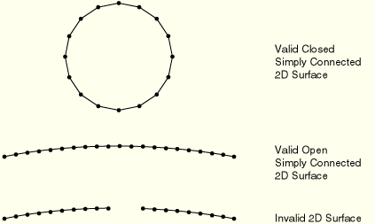
A contact pair surface cannot be made up of two or more disconnected regions. The definition of analytical rigid surfaces automatically ensures that these surfaces are continuous. However, care must be taken to define surfaces formed with elements so that they are continuous across element edges in three-dimensional models or through nodes in two-dimensional models. This continuity requirement has several implications for what constitutes a valid or invalid surface definition. In two dimensions the surface must be either a simple, nonintersecting curve with two terminal ends or a closed loop. Figure 29.4.1–2 shows examples of valid and invalid two-dimensional surfaces for use in contact pairs.
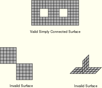
In three dimensions an edge of an element face belonging to a valid surface may be either on the perimeter of the surface or shared by one other face. Two element faces forming a contact pair surface cannot be joined just at a shared node; they must be joined across a common element edge. An element edge cannot be shared by more than two surface facets. Figure 29.4.1–3 illustrates valid and invalid three-dimensional surfaces for use in contact pairs.
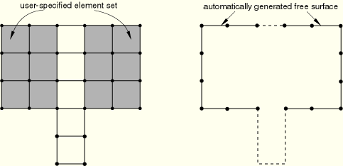
The continuity requirement applies to both automatically generated free surfaces and surfaces defined with element face identifiers (see “Defining element-based surfaces,” Section 2.3.2). Figure 29.4.1–4 shows an automatically generated free surface resulting from the specification of an element set consisting of two disjointed groups of elements. The resulting surface is not continuous since it is composed of two disjoint open curves.
The following restrictions apply when defining a contact simulation for two-dimensional (planar) or axisymmetric problems:
A contact pair cannot involve a planar surface and an axisymmetric surface. This restriction applies only to deformable and element-based rigid surfaces.
Defining a contact pair that contains two surfaces formed by planar elements of different sizes in the out-of-plane direction (“depth”) is not recommended and will result in a warning message. In such a case frictional stresses are calculated based on a weighted average depth, with the weighting for the first surface equal to the user-specified contact surface weighting factor. The out-of-plane thickness for two-dimensional beam element-based surfaces is always assumed to be one. As a result, the contact pressure acting on such a surface can be considered as a line force as well.
When more than one contact pair involves contact between the same rigid surface formed by planar elements and different planar deforming surfaces, the deforming surfaces must all have the same depth; otherwise, a warning message will be issued. The depth value used for calculating contact stresses will then be taken from one of these deforming surfaces, but this choice cannot be predicted.
Element-based surfaces cannot be formed on three-dimensional beam or truss elements, so node-based surfaces must be used to define a surface on these elements. Because a node-based surface must be used, a surface on three-dimensional beam or truss elements must always form the slave surface in a pure master-slave contact pair. Therefore, it is not possible to have two three-dimensional beam or truss structures contact each other.
There are two tracking approaches for the contact pair algorithm in ABAQUS/Explicit: finite sliding and small sliding. Finite sliding is the most general and allows arbitrary motion of the surfaces forming the contact pair. Small sliding assumes that, although the bodies may undergo large motions, there will be relatively little sliding of one surface along the other. By default, ABAQUS/Explicit uses the finite-sliding approach. Only the finite-sliding approach is available for self-contact or contact involving analytical rigid surfaces.
ABAQUS/Explicit is designed to simulate highly nonlinear events or processes. Because it is possible for a node on one surface to contact any of the facets on the opposite surface, ABAQUS/Explicit must use sophisticated search algorithms for tracking the motions of the surfaces.
The contact search algorithm is designed to be robust, yet computationally efficient. This algorithm assumes that the incremental relative tangential motion between surfaces does not significantly exceed the dimensions of the master surface facets, but there is no limit to the overall relative motion between surfaces. It is rare for the incremental motion to exceed the facet size because of the small time increment used in explicit dynamic analyses. In cases involving relative surface velocities that exceed material wave speeds, it may be necessary to reduce the time increment.
The contact search algorithm uses a global search at the beginning of each step, and a hierarchical global/local search algorithm is used for the other increments. The default contact search algorithm can handle the majority of typical contact situations. However, there are some situations that require special attention. We will consider a pure master-slave contact pair for discussion purposes. For a balanced master-slave contact pair, the contact search computations are performed twice for each contact pair.
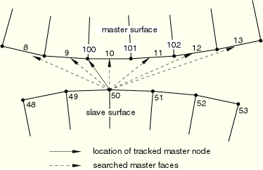
A global search determines the globally nearest master surface facet for each slave node in a given contact pair. A bucket sorting algorithm is used to minimize the computational expense of these searches. A two-dimensional example, without consideration of “buckets,” is shown in Figure 29.4.1–5.
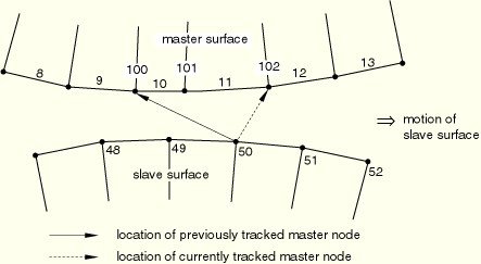
The global search computes the distance from node 50 to all of the master surface facets in the same bucket as node 50. It determines that the nearest facet on the master surface to node 50 is the facet of element 10. Node 100 is the node on this facet that is nearest to node 50, and it is designated the tracked master surface node. This search is conducted for each slave node, comparing each node against all of the facets on the master surface that are in the same bucket. Despite the bucket sorting algorithm, global searches are computationally expensive: performing a global contact search in every increment will more than double the run time of many ABAQUS/Explicit contact analyses.ABAQUS/Explicit uses a local contact search to track the motion of the surfaces during most increments of an analysis. In this approach a given slave node searches only the facets that are attached to the previously tracked master surface node. ABAQUS/Explicit determines which adjacent facet is the nearest to the slave node. It then determines which node on that facet is the closest master surface node to the slave node and updates the tracked master surface node. If the closest master surface node is not the same as the previously tracked master surface node, ABAQUS/Explicit performs another iteration of the local search.
In the example shown in Figure 29.4.1–6, node 50 moves as shown during an increment. In the first iteration of the search ABAQUS/Explicit finds that the master surface facet on element 10 is still the closest facet of those attached to node 100 but that node 101 is now the tracked master surface node. Because the previously tracked node was node 100, ABAQUS/Explicit performs another iteration. In this second iteration a new element, element 11, is found to be the closest facet and the closest master surface node is 102. Another iteration is performed because the identity of the tracked master surface node changed. In the third iteration the identity of the tracked node does not change, so ABAQUS/Explicit designates node 102 as the tracked master surface node for slave node 50.
A local search is substantially less expensive computationally than a global search.
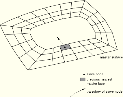
By default for two-surface contact pairs, ABAQUS/Explicit performs a more thorough search of the master faces near each slave node every one hundred increments, which is sufficient for most analyses. However, there are some valid contact situations where a global search needs to be used more or less often during the step. Figure 29.4.1–7 illustrates a situation that might require more frequent global tracking. The master surface is a valid surface, but it contains a hole. The slave node shown identifies the shaded element facet as the closest master surface facet during an increment. The local contact search looks at this master surface facet and its neighbors.
If the slave node displaces across the hole in relatively few increments, the potential contact between the slave node and the master surface facets across the hole will not be detected because the local contact search will still be checking the shaded facet. This same situation can occur when a slave node moves rapidly across a deep valley in the master surface. The solution to this problem is to conduct global contact searches more frequently. You can specify the number of increments between global searches, n, for a given contact pair, if a value other than the default of 100 is desired.
| Input File Usage: | Use both of the following options: |
*CONTACT PAIR, CPSET=contact_pair_set_name *CONTACT CONTROLS, CPSET=contact_pair_set_name, GLOBTRKINC=n |
| ABAQUS/CAE Usage: | Interaction module: Create Contact Controls: Name: contact_controls_name, ABAQUS/Explicit contact controls: Specify max number of increments: n |
Interaction editor: Contact controls: contact_controls_name |
ABAQUS/Explicit uses similar contact searching methods for simulations with self-contact as for two-surface contact; however, more frequent global searches are often necessary for self-contact problems. By default, contact pairs with self-contact use a global contact search every four increments, compared to every 100 increments for two-surface contact pairs. If several facets that are unconnected to each other are found to be near a slave node during global tracking, global tracking automatically will be performed more frequently than the specified number of increments. Despite this precaution, the self-contact algorithm will be less robust if n is specified to be significantly greater than the default.
The default local contact search used by ABAQUS/Explicit uses techniques that allow it to use a minimum amount of computational time. If the local contact search has difficulty enforcing the appropriate contact conditions, a more conservative local contact search may resolve the problem. The contact search specified has no effect on contact pairs using self-contact.
| Input File Usage: | Use both of the following options: |
*CONTACT PAIR, CPSET=contact_pair_set_name *CONTACT CONTROLS, CPSET=contact_pair_set_name, FASTLOCALTRK=NO |
| ABAQUS/CAE Usage: | Interaction module:
Create Contact Controls: Name: contact_controls_name,
ABAQUS/Explicit contact controls: toggle off Fast local tracking |
When the small-sliding or infinitesimal-sliding contact approach is invoked (see “Sliding formulation” in “Contact formulation for ABAQUS/Explicit contact pairs,” Section 29.4.4), ABAQUS/Explicit performs a single global search at the beginning of the first step to determine the globally nearest master surface facet for each slave node in the given contact pair. Once the nearest facet has been determined, the nearest point on that facet defines the anchor point. Contact constraints will not be applied to slave nodes that do not project onto any master surface facet. No further tracking is performed during the step or for subsequent steps in which the contact pair remains active. This makes the small-sliding/infinitesimal-sliding contact approach less expensive computationally than the finite-sliding contact approach. The cost savings are most significant for three-dimensional contact problems.
You can write the contact surface variables associated with the interaction of contact pairs to the ABAQUS output database (.odb) file. The surface variables for a mechanical contact analysis include contact pressure and force, frictional shear stress and force, relative tangential motion (slip) of the surfaces during contact, the status of bonded nodes, whole surface resultant quantities (i.e., force, moment, center of pressure, and total area in contact), and the maximum torque transmitted about the z-axis of axisymmetric elements.
The generic variables CSTRESS, CFORCE, FSLIP, and FSLIPR are valid field output requests for ABAQUS/Explicit. If CSTRESS is requested for a contact pair, the variables CPRESS (contact pressure), CSHEAR1 (contact traction in the local 1-direction), and, if the contact interaction is three-dimensional, CSHEAR2 (contact traction in the local 2-direction) can be contoured in ABAQUS/CAE for each discrete (i.e., non-analytical) surface in a contact pair.
Contours of contact pressure (CPRESS) on surfaces used with the contact pair algorithm will be displayed using the convention that a positive pressure represents compressive contact on the positive side of the surface. The positive side of the surface can be determined by drawing the surface normals in the Visualization module of ABAQUS/CAE. Following this convention, the sign of CPRESS will be reversed for contact on the negative (back) side of a double-sided surface, so negative values of CPRESS may be seen if contact occurs on the back side of a double-sided surface. If contact from separate contact pairs occurs on both sides of the double-sided surface at the same point, the value of CPRESS is given for each contact pair separately.
If CFORCE is requested for a contact pair, the variables CNORMF (normal contact force) and CSHEARF (shear contact force) can be plotted as vectors in a symbol plot in ABAQUS/CAE for each discrete (i.e., non-analytical) surface in a contact pair.
If FSLIPR is requested, FSLIPR (the magnitude of the slip rate for slave nodes in contact) can be contoured in ABAQUS/CAE for each slave surface in a contact pair. In addition, for three-dimensional contact interactions involving an analytical rigid surface and for all two-dimensional contact interactions, components of net slip rate based on local tangent directions (FSLIPR1 and, in three dimensions, FSLIPR2) can also be contoured in ABAQUS/CAE for each slave surface in a contact pair if FSLIPR is requested. All of the slip rate variables associated with FSLIPR are zero whenever a slave node is not in contact.
If FSLIP is requested, FSLIPEQ (the length of the overall slip path for a slave node while it is in contact) can be contoured in ABAQUS/CAE for each slave surface in a contact pair. In addition, for three-dimensional contact interactions involving an analytical rigid surface and for all two-dimensional contact interactions, components of net slip (FSLIP1 and, in three dimensions, FSLIP2) can also be contoured in ABAQUS/CAE for each slave surface in a contact pair if FSLIP is requested. These slip variables are equivalent to the slip rate variables integrated over time: FSLIPEQ, FSLIP1, and FSLIP2 are equivalent to FSLIPR, FSLIPR1, and FSLIPR2 integrated over time, respectively. Therefore, these slip variables account only for relative motions that occur while slave nodes are in contact.
Detailed history output on the status of bonded surfaces is available from an ABAQUS/Explicit simulation. Details can be found in “Breakable bonds,” Section 30.1.9.
Several whole surface contact variables are available as history output. These variables record the contact state of a surface as a set of force (CFN, CFS, and CFT) and moment (CMN, CMS, and CMT) resultants with respect to the origin. Additional variables give the total area (CAREA, defined as the sum of all the facets where there is contact force) in contact at a given time and the center of pressure (XN, XS, and XT) on the surface (defined as the point closest to the centroid of the surface that lies on the line of action of the resultant force for which the resultant moment is zero). The last letter of each variable name (except the variable CAREA) denotes which contact force distribution on the surface is used to calculate the resultant: the letter N denotes that the normal contact forces are used to derive the resultant quantity; the letter S denotes that the shear contact forces are used to derive the resultant quantity; and the letter T denotes that the sum of the normal and shear contact forces are used to derive the resultant quantity.
When modeling surface-based contact with axisymmetric (CAX) elements, ABAQUS/Explicit can calculate the maximum torque (output variable CTRQ) that can be transmitted about the z-axis. The maximum torque, T, is defined as
![]()
Additional discussion on requesting contact surface output can be found in “Surface output” in “Output to the output database,” Section 4.1.3. Output from thermal interactions is discussed in “Thermal contact properties,” Section 30.2.1.