Products: ABAQUS/Standard ABAQUS/CAE
Contact pairs in ABAQUS/Standard:
can be used to define interactions between bodies in mechanical, coupled temperature-displacement, coupled pore pressure-displacement, coupled thermal-electrical, and heat transfer simulations;
are part of the model definition;
can be formed using a pair of rigid or deformable surfaces or a single deformable surface;
do not have to use surfaces with matching meshes; and
cannot be formed with one two-dimensional surface and one three-dimensional surface.
You can define contact in ABAQUS/Standard in terms of two surfaces that may interact with each other as a “contact pair,” or in terms of a single surface that may interact with itself in “self-contact.” ABAQUS/Standard enforces contact conditions by forming equations involving groups of nearby nodes from the respective surfaces or, in the case of self-contact, from separate regions of the same surface. After the selection of contact pair surfaces, three key factors must be determined when creating a contact formulation:
the contact discretization;
the tracking approach; and
the assignment of “master” and “slave” roles to the respective surfaces.
Before defining contact, you must select the surfaces for the contact pair. ABAQUS/Standard applies conditional constraints at various locations on each surface to simulate contact conditions. The locations and conditions of these constraints depend on the contact discretization used in the overall contact formulation. ABAQUS/Standard offers two contact discretization options: a traditional “node-to-surface” discretization and a true “surface-to-surface” discretization.
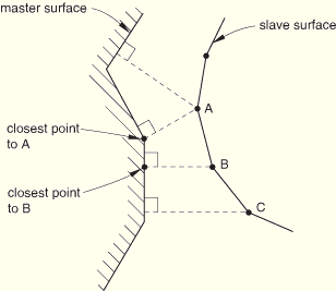
With traditional node-to-surface discretization the contact conditions are established such that each “slave” node on one side of a contact interface effectively interacts with a point of projection on the “master” surface on the opposite side of the contact interface (see Figure 29.2.1–1). Thus, each contact condition involves a single slave node and a group of nearby master nodes from which values are interpolated to the projection point.
Traditional node-to-surface discretization has the following characteristics:
The slave nodes are constrained not to penetrate into the master surface; however, the nodes of the master surface can, in principle, penetrate into the slave surface (for example, see the case on the upper-right of Figure 29.2.1–2).
The contact direction is based on the normal of the master surface.
The only information needed for the slave surface is the location and surface area associated with each node; the direction of the slave surface normal and slave surface curvature are not relevant. Thus, the slave surface can be defined as a group of nodes—a node-based surface.
Node-to-surface discretization is available even if a node-based surface is not used in the contact pair definition.
To optimize stress accuracy, surface-to-surface discretization considers the shape of both the slave and master surfaces in the region of contact constraints. Figure 29.2.1–3 shows an example of improved contact pressure accuracy with surface-to-surface contact as compared to node-to-surface contact.
Figure 29.2.1–3 Comparison of contact pressure accuracy for node-to-surface and surface-to-surface contact discretizations.

Surface-to-surface discretization has the following key characteristics:
Contact conditions are enforced in an average sense over the slave surface, rather than at discrete points (such as at slave nodes, as in the case of node-to-surface discretization). Therefore, some penetration may be observed at individual nodes; however, large, undetected penetrations of master nodes into the slave surface do not occur with this discretization. Figure 29.2.1–2 compares contact enforcement for node-to-surface and surface-to-surface contact for an example with dissimilar mesh refinement on the contacting bodies.
Surface-to-surface discretization is not applicable if a node-based surface is used in the contact pair definition.
Surface-to-surface discretization generally involves more nodes per constraint and can, therefore, increase solution cost. In most applications the extra cost is fairly small, but the cost can become significant in some cases. The following factors (especially in combination) can lead to surface-to-surface contact being costly:
A large fraction of the model is involved in contact.
The master surface is more refined than the slave surface.
Multiple layers of shells are involved in contact, such that the master surface of one contact pair acts as the slave surface of another contact pair.
In ABAQUS/Standard there are two tracking approaches to account for the relative motion of the two surfaces forming a contact pair in mechanical contact simulations.
Finite-sliding contact is the most general tracking approach and allows for arbitrary relative separation, sliding, and rotation of the contacting surfaces. For finite-sliding contact the connectivity of the currently active contact constraints changes upon relative tangential motion of the contacting surfaces. For a detailed description of how ABAQUS/Standard calculates finite-sliding contact, see “Using the finite-sliding tracking approach” in “Contact formulation for ABAQUS/Standard contact pairs,” Section 29.2.2.
Small-sliding contact assumes there will be relatively little sliding of one surface along the other and is based on linearized approximations of the master surface per constraint. The groups of nodes involved with individual contact constraints are fixed throughout the analysis for small-sliding contact, although the active/inactive status of these constraints typically can change during the analysis. You should consider using small-sliding contact when the approximations are reasonable, due to computational savings and added robustness. For a detailed description of how ABAQUS/Standard calculates small-sliding contact, see “Using the small-sliding tracking approach” in “Contact formulation for ABAQUS/Standard contact pairs,” Section 29.2.2.
Your choice of contact discretization and tracking approach have considerable impact on an analysis. In addition to the qualities already discussed, certain combinations of discretizations and tracking approaches have their own characteristics and limitations associated with them. These characteristics are summarized in Table 29.2.1–1. You should also consider the solution costs associated with the various contact formulations.
Table 29.2.1–1 Comparison of contact formulation characteristics.
| Characteristic | Contact formulation | |||
|---|---|---|---|---|
| Node-to-surface | Surface-to-surface | |||
| Finite-sliding | Small-sliding | Finite-sliding | Small-sliding | |
| Account for shell thickness by default | No | Yes | Yes | Yes |
| Allow self-contact | Yes | No | Yes | No |
| Allow double-sided surfaces | No | No | No | Yes |
| Smooth master surface by default | Yes | Yes for anchor points; each constraint uses flat approximation of master surface | No | No for anchor points; each constraint uses flat approximation of master surface |
| Default constraint enforcement method | Augmented Lagrange method for 3-D self-contact; otherwise, direct method | Direct method | Penalty method | Direct method |
Most contact formulations will account for the surface thickness of a shell when calculating contact constraints. However, the finite-sliding, node-to-surface formulation will not account for shell thicknesses. These calculations are discussed in more detail in “Accounting for shell and membrane thickness” in “Contact formulation for ABAQUS/Standard contact pairs,” Section 29.2.2.
Self-contact is typically the result of large deformation in a model. It is often difficult to predict which regions will be involved in the contact or how they will move relative to each other. Therefore, self-contact cannot use the small-sliding tracking approach.
Most contact formulations involving shell-like surfaces require the use of single-sided surfaces. However, the small-sliding, surface-to-surface formulation does allow for double-sided surfaces. See “Orientation considerations for shell-like surfaces” later in this section for more information.
When using node-to-surface discretization, corners or small protrusions of a jagged master surface are allowed to penetrate the spaces between nodes in the node-based surface. It is sometimes possible for a slave node sliding along the master surface to snag on these corners. Therefore, ABAQUS/Standard automatically smooths the master surface for contact calculations utilizing node-to-surface discretization to minimize this phenomenon. The details are discussed further in “Smoothing master surfaces for the finite-sliding, node-to-surface formulation” in “Contact formulation for ABAQUS/Standard contact pairs,” Section 29.2.2.
When using surface-to-surface discretization, ABAQUS/Standard accounts for the spaces between nodes on both the master and slave surfaces, so snagging is not a problem. No smoothing of the master surface occurs when using surface-to-surface discretization. However, surface-to-surface discretization considers contact conditions in an average sense over a finite region; as a result, the surface-to-surface contact calculations introduce some inherent smoothing characteristics at the constraint level.
For most contact formulations ABAQUS/Standard strictly enforces the contact constraints discussed previously by default. However, this can sometimes lead to excessive constraints and convergence difficulty with certain contact formulations. ABAQUS/Standard will utilize numerical techniques that allow for a “softened” enforcement of the contact constraints in these situations. The numerical constraint enforcement methods are discussed in detail in “Constraint enforcement methods for ABAQUS/Standard contact pairs,” Section 29.2.3.
The cost of contact calculations in each iteration of an analysis is roughly proportional to the number of constraints imposed by the contact formulation, as well as the number of nodes involved in each constraint. In general, node-to-surface contact is less costly per iteration than surface-to-surface contact. For node-to-surface contact, the number of potential constraints is proportional to the number of slave nodes, and each constraint involves a single slave node and a group of nearby master nodes. For surface-to-surface contact, the constraints depend on the tracking approach:
For finite-sliding, surface-to-surface contact, the number of potential constraints is proportional to the number of slave faces and is generally greater than the number of slave nodes. The constraints are located within the slave faces rather than at slave nodes. Each constraint involves multiple slave and master nodes.
For small-sliding, surface-to-surface contact, the number of potential constraints is proportional to the number of slave nodes. Each constraint involves a single slave node and a group of nearby master nodes (which is also true with node-to-surface contact). However, the faces around the slave nodes are also considered, so the number of master nodes per constraint tends to be greater in this case than with small-sliding, node-to-surface contact.
Regardless of whether finite- or small-sliding, node-to-surface or surface-to-surface contact is used, ABAQUS/Standard enforces the following rules related to the assignment of the master and slave roles for contact surfaces:
Analytical rigid surfaces and rigid-element-based surfaces must always be the master surface.
A node-based surface can act only as a slave surface and always uses node-to-surface contact.
Slave surfaces must always be attached to deformable bodies or deformable bodies defined as rigid.
Both surfaces in a contact pair cannot be rigid surfaces with the exception of deformable surfaces defined as rigid (see “Rigid body definition,” Section 2.4.1).
When both surfaces in a contact pair are element-based and attached to either deformable bodies or deformable bodies defined as rigid, you have to choose which surface will be the slave surface and which will be the master surface. This choice is particularly important for node-to-surface contact. Generally, if a smaller surface contacts a larger surface, it is best to choose the smaller surface as the slave surface. If that distinction cannot be made, the master surface should be chosen as the surface of the stiffer body or as the surface with the coarser mesh if the two surfaces are on structures with comparable stiffnesses. The stiffness of the structure and not just the material should be considered when choosing the master and slave surface. For example, a thin sheet of metal may be less stiff than a larger block of rubber even though the steel has a larger modulus than the rubber material. If the stiffness and mesh density are the same on both surfaces, the preferred choice is not always obvious.
Compared with node-to-surface contact, the choice of master and slave surfaces for surface-to-surface contact typically has much less effect on the results. However, the assignment of master and slave roles can have a significant effect on performance with surface-to-surface contact if the two surfaces have dissimilar mesh refinement; the solution can become quite expensive if the slave surface is much coarser than the master surface.
To define a contact pair, you must indicate which pairs of surfaces may interact with one another or which surface may interact with itself, as well as specify a contact formulation. Every contact pair must also refer to an interaction property. Interaction property definitions are discussed later in this section in “Assigning a surface interaction definition to a contact pair.”
When a contact pair contains two surfaces, the master and slave surfaces are not allowed to include any of the same nodes and you must choose which surface will be the slave and which will be the master.
ABAQUS/Standard uses a finite-sliding, node-to-surface formulation by default.
| Input File Usage: | *CONTACT PAIR, INTERACTION=interaction_property_name slave_surface_name, master_surface_name |
You can also specify the contact discretization directly: *CONTACT PAIR, INTERACTION=interaction_property_name, TYPE=NODE TO SURFACE slave_surface_name, master_surface_name |
| ABAQUS/CAE Usage: | Interaction module: Create Interaction: Surface-to-surface contact (Standard): select the master surface, click Surface or Node Region, select the slave surface, Interaction editor, Sliding formulation: Finite sliding, Constraint enforcement method: Node to surface, Contact interaction property: interaction_property_name |
A node-based slave surface precludes the use of surface-to-surface discretization. Some contact capabilities are not available with the finite-sliding, surface-to-surface formulation, including pressure penetration loading (see “Pressure penetration loading,” Section 30.1.7) and crack propagation (see “Crack propagation analysis,” Section 11.4.3).
| Input File Usage: | *CONTACT PAIR, INTERACTION=interaction_property_name, TYPE=SURFACE TO SURFACE slave_surface_name, master_surface_name |
| ABAQUS/CAE Usage: | Interaction module: Create Interaction: Surface-to-surface contact (Standard): select the master surface, click Surface, select the slave surface, Interaction editor, Sliding formulation: Finite sliding, Constraint enforcement method: Surface to surface, Contact interaction property: interaction_property_name |
The small-sliding tracking approach uses node-to-surface discretization by default. For an explanation of when the small-sliding tracking approach is appropriate in an analysis, see “Using the small-sliding tracking approach” in “Contact formulation for ABAQUS/Standard contact pairs,” Section 29.2.2.
| Input File Usage: | *CONTACT PAIR, INTERACTION=interaction_property_name, SMALL SLIDING slave_surface_name, master_surface_name |
You can also specify the contact discretization directly: *CONTACT PAIR, INTERACTION=interaction_property_name, SMALL SLIDING, TYPE=NODE TO SURFACE slave_surface_name, master_surface_name |
| ABAQUS/CAE Usage: | Interaction module: Create Interaction: Surface-to-surface contact (Standard): select the master surface, click Surface or Node Region, select the slave surface, Interaction editor, Sliding formulation: Small sliding, Constraint enforcement method: Node to surface, Contact interaction property: interaction_property_name |
A node-based slave surface precludes the use of surface-to-surface discretization.
| Input File Usage: | *CONTACT PAIR, INTERACTION=interaction_property_name, SMALL SLIDING, TYPE=SURFACE TO SURFACE slave_surface_name, master_surface_name |
| ABAQUS/CAE Usage: | Interaction module: Create Interaction: Surface-to-surface contact (Standard): select the master surface, click Surface, select the slave surface, Interaction editor, Sliding formulation: Small sliding, Constraint enforcement method: Surface to surface, Contact interaction property: interaction_property_name |
For node-to-surface contact it is possible for master surface nodes to penetrate the slave surface without resistance with the strict master-slave algorithm used by ABAQUS/Standard. This penetration tends to occur if the master surface is more refined than the slave surface or a large contact pressure develops between soft bodies. Refining the slave surface mesh often minimizes the penetration of the master surface nodes. If the refinement technique does not work or is not practical, a symmetric master-slave method can be used if both surfaces are element-based surfaces with deformable or deformable-made-rigid parent elements. To use this method, define two contact pairs using the same two surfaces, but switch the roles of master and slave surface for the two contact pairs. This method causes ABAQUS/Standard to treat each surface as a master surface and, thus, involves additional computational expense because contact searches must be conducted twice for the same contact pair. The increased accuracy provided by this method must be compared to the additional computational cost.
All of the contact formulations are available for symmetric master-slave contact pairs, and can be applied using the same options discussed above.
| Input File Usage: | *CONTACT PAIR, INTERACTION=interaction_property_name surface_1, surface_2 surface_2, surface_1 |
| ABAQUS/CAE Usage: | Interaction module: Create Interaction: Surface-to-surface
contact (Standard): select the master surface, click Surface, select the slave surface |
It can be difficult to interpret the results at the interface for symmetric master-slave contact pairs. In single master-slave contact pairs the results are reported only for the slave surface. In symmetric master-slave contact pairs both surfaces are slave surfaces, so each has results associated with it. The problem is that the results for contact pressure are not independent of each other; the contact pressure on one surface will not necessarily be equivalent to the pressure on the other. The total contact pressure acting on both surfaces is the sum of the contact pressures on each side of the interface.
When symmetric master-slave contact pairs are used in a finite-sliding simulation, it is possible that ABAQUS/Standard will report one of the surfaces as open and the other as closed. Typically this is caused by the shape or relative mesh refinement of the two surfaces. In two-dimensional finite-sliding problems, smoothing of the master surface may also play a role.
Using symmetric master-slave contact pairs can lead to overconstraint problems when very stiff or “hard” contact conditions are enforced. See “Constraint enforcement methods for ABAQUS/Standard contact pairs,” Section 29.2.3, for a discussion of overconstraints and alternate constraint enforcement methods.
The division of contact pressure between the two symmetric surfaces discussed above can cause inaccurate modeling of frictional behavior. Frictional slip is calculated independently for each surface based on the contact pressure for that surface and the friction coefficient. Limits on the frictional shear stress, such as the optional equivalent shear stress limit that you can specify for the friction model (see “Using the optional shear stress limit” in “Frictional behavior,” Section 30.1.5), will not be applied correctly because the contact pressure acting on each surface will be less than the contact pressure calculated with a single master-slave contact pair.
Define contact between a single surface and itself by specifying only a single surface or by specifying the same surface twice. The small-sliding tracking approach cannot be used with self-contact.
ABAQUS/Standard uses node-to-surface contact discretization by default for self-contact.
| Input File Usage: | Use either of the following options: |
*CONTACT PAIR, INTERACTION=interaction_property_name
surface_1,
*CONTACT PAIR, INTERACTION=interaction_property_name surface_1, surface_1 |
| ABAQUS/CAE Usage: | Interaction module: Create Interaction: Self-contact (Standard): select the surface Interaction editor, Contact interaction property: interaction_property_name, Constraint enforcement method: Node to surface |
or Interaction module: Create Interaction: Surface-to-surface contact (Standard): select the surface, click Surface, select the surface again Interaction editor, Sliding formulation: Finite sliding, Constraint enforcement method: Node to surface, Contact interaction property: interaction_property_name |
Surface-to-surface discretization often leads to more accurate modeling of self-contact simulations. However, because the self-contact surface is acting as both a master and a slave, surface-to-surface discretization can sometimes significantly increase the solution cost.
| Input File Usage: | Use either of the following options: |
*CONTACT PAIR, INTERACTION=interaction_property_name, TYPE=SURFACE TO SURFACE
surface_1,
*CONTACT PAIR, INTERACTION=interaction_property_name, TYPE=SURFACE TO SURFACE surface_1, surface_1 |
| ABAQUS/CAE Usage: | Interaction module: Create Interaction: Self-contact (Standard): select the surface Interaction editor, Contact interaction property: interaction_property_name, Constraint enforcement method: Surface to surface |
or Interaction module: Create Interaction: Surface-to-surface contact (Standard): select the surface, click Surface, select the surface again Interaction editor, Sliding formulation: Finite sliding, Constraint enforcement method: Surface to surface, Contact interaction property: interaction_property_name |
Self-contact is valid only for mechanical surface interactions and is limited to finite sliding with element-based surfaces.
Since a node of a self-contacting surface can be both a slave node and a member of the master surface, contact behavior is very similar to symmetric master-slave contact pairs. The characteristics described in “Using symmetric master-slave contact pairs to improve contact modeling” above apply in this case, including the issue of overconstraints. In the special case of two-dimensional self-contact the nodes adjacent to a vertex where a surface folds over on itself follow a strict master-slave algorithm to avoid overconstraints. ABAQUS/Standard automatically applies some numerical “softening” to the contact conditions with most self-contact formulations. See “Constraint enforcement methods for ABAQUS/Standard contact pairs,” Section 29.2.3, for a discussion of the numerical constraint enforcement methods used with self-contact.
A surface interaction definition specifies the constitutive contact properties and the constraint enforcement methods used by a contact pair. Every contact pair in a model must refer to a surface interaction definition, even if the contact pair uses the default contact property models. See “Mechanical contact properties: overview,” Section 30.1.1, for information on defining contact properties. A non-default constraint enforcement method can be specified as part of a surface interaction definition, as described in “Constraint enforcement methods for ABAQUS/Standard contact pairs,” Section 29.2.3.
Multiple contact pairs can refer to the same surface interaction definition.
| Input File Usage: | Use both of the following options: |
*CONTACT PAIR, INTERACTION=interaction_property_name *SURFACE INTERACTION, NAME=interaction_property_name |
| ABAQUS/CAE Usage: | Interaction module: |
Create Interaction Property: Name: interaction_property_name, Contact Interaction editor: Contact interaction property: interaction_property_name |
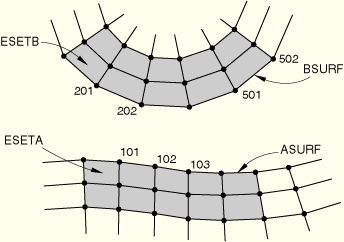
Figure 29.2.1–4 shows the mesh used in this example. For purposes of this example, the surface ASURF is the slave surface of the contact pair. The property definition for the contact pair (GRATING) uses the finite-sliding, node-to-surface formulation with a friction model with ![]() =0.4 and uses the default “hard” contact model for the behavior normal to the surfaces.
=0.4 and uses the default “hard” contact model for the behavior normal to the surfaces.
*HEADING
…
*SURFACE, NAME=ASURF
ESETA,
*SURFACE, NAME=BSURF
ESETB,
*CONTACT PAIR, INTERACTION=GRATING
ASURF, BSURF
*SURFACE INTERACTION, NAME=GRATING
*FRICTION
0.4
*NSET, NSET=SNODES
101, 102, 103
*STEP, NLGEOM
…
*END STEP
Methods for creating surfaces are discussed in “Defining element-based surfaces,” Section 2.3.2; “Defining node-based surfaces,” Section 2.3.3; and “Defining analytical rigid surfaces,” Section 2.3.4. Those sections discuss general restrictions for the various surface types. Additional restrictions and considerations for surfaces used in contact definitions are discussed below; in some cases these factors depend on the contact formulation that you specify.
ABAQUS/Standard requires master contact surfaces to be single-sided in all cases except for small-sliding, surface-to-surface contact. This requires that you consider the proper orientation for master surfaces defined on elements, such as shells and membranes, that have positive and negative directions. For node-to-surface contact the orientation of slave surface normals is irrelevant, but for surface-to-surface contact the orientation of single-sided slave surfaces is taken into consideration.
Double-sided element-based surfaces are allowed for small-sliding, surface-to-surface contact, although they are not always appropriate for cases with deep initial penetrations. If the master and slave surfaces are both double-sided, the positive or negative orientation of the contact normal direction will be chosen such as to minimize (or avoid) penetrations for each contact constraint. If either or both of the surfaces are single-sided, the positive or negative orientation of the contact normal direction will be determined from the single-sided surface normals rather than the relative positions of the surfaces.
When the orientation of a contact surface is relevant to the contact formulation, you must consider the following aspects for surfaces on structural (beam and shell), membrane, truss, or rigid elements:
Adjacent surface faces must have consistent normal directions. ABAQUS/Standard will issue an error message if adjacent surface faces have inconsistent normals on a single-sided surface whose orientation is relevant to the contact formulation.
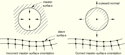
Except for initial interference fit problems (see “Modeling contact interference fits in ABAQUS/Standard,” Section 29.2.4), the slave surface should be on the same side of the master surface as the outward normal. If, in the initial configuration, the slave surface is on the opposite side of the master surface as the outward normal, ABAQUS/Standard will detect overclosure of the surfaces and may have difficulty finding an initial solution if the overclosure is severe. An improper specification of the outward normal will often cause an analysis to immediately fail to converge. Figure 29.2.1–5 illustrates the proper and improper specification of a master surface's outward normal.
Contact will be ignored with surface-to-surface discretization if single-sided slave and master surfaces have normal directions that are in approximately the same direction (for example, contact will not be enforced if the dot product of the slave and master surface normals is positive).
Initial clearances can be displayed in ABAQUS/CAE with a contour plot of the variable COPEN at increment 0 of the first step; initial overclosures correspond to negative clearances.
ABAQUS/Standard provides a detailed printout of the model's initial contact state.
In addition to the orientation restrictions discussed above, certain connectivity restrictions apply to contact surfaces depending on the type of contact formulation. Surface connectivity restrictions for the various contact formulations are summarized in Table 29.2.1–2. As indicated in this table, the connectivity restrictions are sometimes different for master and slave surfaces. Self-contact surfaces act as both master and slave surfaces; therefore, if a restriction applies to either a master or slave surface, it also applies to self-contact. The potential connectivity restrictions referred to in Table 29.2.1–2 are described below:
Table 29.2.1–2 Summary of which connectivity characteristics of element-based surfaces are allowed for various contact formulations.
| Contact formulation | Connectivity characteristics | |
|---|---|---|
| Discontinuous (or 3-D faces joined at only one node) | T-intersection | |
| Finite-sliding, node-to-surface | Master: Not allowed Slave: Allowed | Master: Not allowed Slave: Allowed |
| Small-sliding, node-to-surface | Master: Allowed Slave: Allowed | Master: Not allowed Slave: Allowed |
| Finite-sliding, surface-to-surface | Master: Allowed Slave: Allowed | Master: Not allowed Slave: Not allowed |
| Small-sliding, surface-to-surface | Master: Allowed Slave: Allowed | Master: Allowed Slave: Allowed |
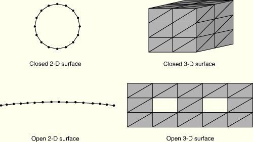
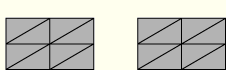
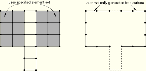
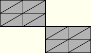
Discontinuous surfaces: Discontinuous contact surfaces are allowed in many cases, but the master surface for finite-sliding, node-to-surface contact cannot be made up of two or more disconnected regions (they must be continuous across element edges in three-dimensional models or across nodes in two-dimensional models). Figure 29.2.1–6 shows examples of continuous surfaces, whereas Figure 29.2.1–7 and Figure 29.2.1–8 show examples of discontinuous surfaces. Figure 29.2.1–9 shows an automatically generated free surface resulting from the specification of an element set consisting of two disjointed groups of elements. The resulting surface is not continuous since it is composed of two disjoint open curves, so this surface would be invalid as a master surface for finite-sliding, node-to-surface contact.
Portions of three-dimensional surfaces joined at only one node: The finite-sliding, node-to-surface contact formulation also does not allow three-dimensional master surface faces to be joined at a single node (they must be joined across a common element edge). Figure 29.2.1–10 shows an example of a surface with two faces connected by a single node.
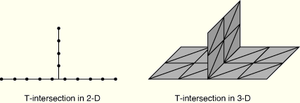
Surfaces with T-intersections: In some cases a contact surface cannot have more than two surface faces sharing a common master node in two dimensions or a common master edge in three dimensions. For example, Figure 29.2.1–11 shows examples of surfaces with T-intersections, in which three faces share a common node in two dimensions or a common edge in three dimensions.
ABAQUS/Standard cannot use three-dimensional beams or trusses to form a master surface because the elements do not have enough information to create unique surface normals. However, these elements can be used to define a slave surface. Two-dimensional beams and trusses can be used to form both master and slave surfaces.
Edge-based surfaces (“Defining element-based surfaces,” Section 2.3.2) on three-dimensional shell elements cannot be used in a contact analysis in ABAQUS/Standard.
Use node-based surfaces with caution when the contact property definition includes user-defined softened contact properties or thermal or electrical interactions because the contact constitutive behavior (which relies on accurate calculation of contact pressure, heat flux, or electric current) will not be enforced correctly unless the precise surface area is associated with each node. For details, see “Contact pressure-overclosure relationships,” Section 30.1.2; “Thermal contact properties,” Section 30.2.1; or “Electrical contact properties,” Section 30.3.1.
You can write the contact surface variables associated with the interaction of contact pairs to the ABAQUS/Standard data (.dat), results (.fil), and output database (.odb) files. All contact pair results are given at the constraint points of the slave surface. The constraint points correspond to the slave nodes except in the case of finite-sliding, surface-to-surface contact, in which case each slave facet contains multiple constraint points.
You can:
request output associated with a given contact pair;
request output associated with a given slave surface, including contributions from all of the contact pairs to which the slave surface belongs; and
limit the output by specifying a node set containing a subset of the nodes on the slave surface except in the case of finite-sliding, surface-to-surface contact.
For small-sliding contact problems the contact area is calculated in the input file preprocessor from the undeformed shape of the model; thus, it does not change throughout the analysis, and contact pressures for small-sliding contact are calculated according to this invariant contact area. This behavior is different from that in finite-sliding contact problems, where the contact area and contact pressures are calculated according to the deformed shape of the model.
In an axisymmetric analysis the total forces and moments transmitted between the contacting bodies as a result of contact pressure and frictional stress are computed in the same manner as in a two-dimensional analysis. As a result, the component of the total forces along the r-axis is nonzero, and the components of the total moments include contributions from the total forces along the r-axis.
Recall the example shown in Figure 29.2.1–4 and the corresponding input file excerpt given previously in this section in “Assigning a surface interaction definition to a contact pair.” The following input could be added to that excerpt to request the default printed output for only the slave nodes 101, 102, and 103:
*CONTACT PRINT, SLAVE=ASURF, MASTER=BSURF, NSET=SNODESThis output request creates a table of output variables in the printed data (.dat) file. Each row of the table corresponds to a slave node in node set SNODES. The first column of the table identifies the slave node for that row. Because this is a mechanical contact simulation, the second column specifies the contact status at the slave node. Since the contact property definition includes frictional properties, the contact status may be open (OP), closed and sticking tangentially (ST), or closed and sliding tangentially (SL). The remaining columns contain the surface variables requested. In this example the default variables—contact pressure, contact opening, frictional shear stress, and relative tangential slip—were requested. This output request produces the following table in the data file:
CONTACT OUTPUT FOR SLAVE SURFACE ASURF AND MASTER SURFACE BSURF
   NODE  STATUS  CPRESS      CSHEAR1      COPEN       CSLIP1
    101  OP       0.       -4.5870E-14        0.66    -0.24
    102  ST       6.59     -2.585      -3.3168E-14    -0.4598
    103  SL       4.32     -1.73       -2.6276E-13    -0.9946
The OP status indicates that the slave node is not in contact with the master surface. In the sample output above, node 101 is open and, consequently, the contact pressure variable CPRESS is zero. The COPEN variable reports that this node is 0.66 length units away from the master surface.
The ST status indicates that the slave node is in contact with the master surface and is “sticking.” The frictional shear stress acting at the node is below the critical shear stress ![]() , where p is the value of contact pressure shown under CPRESS. In the sample output above, node 102 is sticking since the frictional shear stress CSHEAR1 is below the critical value of 2.64 (0.4 × 6.59). The CSLIP1 variable is the total accumulated (integrated) slip at the slave node. The negative magnitude of CSLIP1 indicates that the node has moved in the negative first slip direction on BSURF. Accumulated slip and slip directions are discussed in more detail below in “Output of tangential motion of the surfaces.”
, where p is the value of contact pressure shown under CPRESS. In the sample output above, node 102 is sticking since the frictional shear stress CSHEAR1 is below the critical value of 2.64 (0.4 × 6.59). The CSLIP1 variable is the total accumulated (integrated) slip at the slave node. The negative magnitude of CSLIP1 indicates that the node has moved in the negative first slip direction on BSURF. Accumulated slip and slip directions are discussed in more detail below in “Output of tangential motion of the surfaces.”
The SL status indicates that the slave node is in contact with the master surface and it is sliding—the frictional shear stress is at the critical shear stress ![]() =
=![]() =
=![]() . In the sample output above, node 103 is sliding, and the frictional shear stress CSHEAR1 is equal to the friction limit 1.73 (0.4 × 4.32).
. In the sample output above, node 103 is sliding, and the frictional shear stress CSHEAR1 is equal to the friction limit 1.73 (0.4 × 4.32).
In the absence of frictional properties when a slave node is in contact with the master surface, its status reads CL for “closed.”
Some details related to this printed output differ for the finite-sliding, surface-to-surface formulation, because the constraints are located within slave facets with that formulation (rather than at slave nodes). This printed output cannot be limited to a specific portion of the slave surface for finite-sliding, surface-to-surface contact. The format of the output in the data file is also somewhat different. Rather than identifying the constraint with a single column giving the slave node number, three columns are needed to identify the constraint: element number (first column), element face identifier (second column), and local constraint point number within a face (third column). For example, two-dimensional surfaces contain two constraint points per face (or segment).
In the example corresponding to Figure 29.2.1–4, additional output variables can also be requested by using the following option:
*CONTACT PRINT, SLAVE=ASURF, MASTER=BSURF, NSET=SNODES
CFN,CFS,CAREA
CMN,CMS
CFT,CMT
XN,XS,XT
Such an output request creates four additional tables of output variables in the printed data (.dat) file. These tables summarize the total forces and moments transmitted between the contacting bodies as a result of contact pressure and frictional stress, the total contact area, and the coordinates of the centers of the contact and frictional forces. The content of each table is given below (the form of this output is the same for finite-sliding, node-to-surface contact):
CONTACT OUTPUT FOR SLAVE SURFACE ASURF AND MASTER SURFACE BSURF
CFNM    CFN1    CFN2    CFN3    CFSM    CFS1    CFS2    CFS3    CAREA
0.608   0.10    0.60      0     0.104   0.10    0.03    0       3.11

CONTACT OUTPUT FOR SLAVE SURFACE ASURF AND MASTER SURFACE BSURF
CMNM    CMN1    CMN2    CMN3    CMSM    CMS1    CMS2    CMS3
0.01    0       0       0.01    0.002   0       0       0.002

CONTACT OUTPUT FOR SLAVE SURFACE ASURF AND MASTER SURFACE BSURF
CFTM    CFT1    CFT2    CFT3    CMTM    CMT1    CMT2    CMT3
0.66    0.20    0.63    0       0.012   0       0       0.012

CONTACT OUTPUT FOR SLAVE SURFACE ASURF AND MASTER SURFACE BSURF
XN1    XN2    XN3    XS1    XS2    XS3    XT1    XT2    XT3
0.1    0      0      0.01   0.02   0      0.11   0.02   0
ABAQUS/Standard provides the relative tangential motion (slip) of the two surfaces at each point on the slave surface as output. In two-dimensional models a slave node can slide along only the master surface in the plane of the model. The tangent to the surfaces in the plane of a two-dimensional model is the first slip direction. ABAQUS/Standard defines the orientation of this tangent by the cross product of the vector into the plane of the model (0., 0., 1.0) and the normal vector. This tangent is the first slip direction of the surface, ![]() . The accumulated incremental relative displacement of the slave surface in this direction is CSLIP1, where the incremental relative displacement is along the current
. The accumulated incremental relative displacement of the slave surface in this direction is CSLIP1, where the incremental relative displacement is along the current ![]() -direction; the
-direction; the ![]() -direction may change during the motion.
-direction may change during the motion.
In a three-dimensional model there are two orthogonal slip directions, ![]() and
and ![]() , for each contact pair. These two directions together with the relevant surface normal form an orthogonal coordinate system at every point on the surface (see “Slip directions for a three-dimensional surface” in “Contact formulation for ABAQUS/Standard contact pairs,” Section 29.2.2, for more details on how slip directions are defined for three-dimensional models). The output variables for the accumulated incremental relative motions along the first and second slip directions are CSLIP1 and CSLIP2, respectively. The incremental relative motions are measured in the current
, for each contact pair. These two directions together with the relevant surface normal form an orthogonal coordinate system at every point on the surface (see “Slip directions for a three-dimensional surface” in “Contact formulation for ABAQUS/Standard contact pairs,” Section 29.2.2, for more details on how slip directions are defined for three-dimensional models). The output variables for the accumulated incremental relative motions along the first and second slip directions are CSLIP1 and CSLIP2, respectively. The incremental relative motions are measured in the current ![]() - and
- and ![]() -directions, which may change during the motion. You can request that the relative motions of surfaces be written as output for an analysis to the data, results, or output database file.
-directions, which may change during the motion. You can request that the relative motions of surfaces be written as output for an analysis to the data, results, or output database file.
ABAQUS/Standard defines the incremental relative motion (slip) for a slave node as the scalar product of the incremental relative nodal displacement vector, ![]() , and a slip direction,
, and a slip direction, ![]() or
or ![]() , associated with the node. The incremental relative nodal displacement vector measures the motion of the slave node relative to the motion of the master surface. Details about the calculation of this quantity can be found in “Small-sliding interaction between bodies,” Section 5.1.1 of the ABAQUS Theory Manual; “Finite-sliding interaction between deformable bodies,” Section 5.1.2 of the ABAQUS Theory Manual; and “Finite-sliding interaction between a deformable and a rigid body,” Section 5.1.3 of the ABAQUS Theory Manual. The sums of all such incremental slips during the analysis are reported as CSLIP1 and CSLIP2. The incremental slip is accumulated only when the slave node is contacting the master surface. In geometrically nonlinear, small- or finite-sliding problems the orientation of the slip directions is updated continually to account for the motion of the surfaces.
, associated with the node. The incremental relative nodal displacement vector measures the motion of the slave node relative to the motion of the master surface. Details about the calculation of this quantity can be found in “Small-sliding interaction between bodies,” Section 5.1.1 of the ABAQUS Theory Manual; “Finite-sliding interaction between deformable bodies,” Section 5.1.2 of the ABAQUS Theory Manual; and “Finite-sliding interaction between a deformable and a rigid body,” Section 5.1.3 of the ABAQUS Theory Manual. The sums of all such incremental slips during the analysis are reported as CSLIP1 and CSLIP2. The incremental slip is accumulated only when the slave node is contacting the master surface. In geometrically nonlinear, small- or finite-sliding problems the orientation of the slip directions is updated continually to account for the motion of the surfaces.
When modeling surface-based contact with axisymmetric elements (type CAX and CGAX elements), ABAQUS/Standard can calculate the maximum torque (output variable CTRQ) that can be transmitted about the z-axis. This capability is often of interest when modeling threaded connectors (see “Axisymmetric analysis of a threaded connection,” Section 1.1.19 of the ABAQUS Example Problems Manual). The maximum torque, T, is defined as
![]()