Products: ABAQUS/Standard ABAQUS/Explicit ABAQUS/CAE
The modified Drucker-Prager/Cap plasticity/creep model:
is intended to model cohesive geological materials that exhibit pressure-dependent yield, such as soils and rocks;
is based on the addition of a cap yield surface to the Drucker-Prager plasticity model (“Extended Drucker-Prager models,” Section 18.3.1), which provides an inelastic hardening mechanism to account for plastic compaction and helps to control volume dilatancy when the material yields in shear;
can be used in ABAQUS/Standard to simulate creep in materials exhibiting long-term inelastic deformation through a cohesion creep mechanism in the shear failure region and a consolidation creep mechanism in the cap region;
can be used in conjunction with either the elastic material model (“Linear elastic behavior,” Section 17.2.1) or, in ABAQUS/Standard if creep is not defined, the porous elastic material model (“Elastic behavior of porous materials,” Section 17.3.1); and
provides a reasonable response to large stress reversals in the cap region; however, in the failure surface region the response is reasonable only for essentially monotonic loading.
The addition of the cap yield surface to the Drucker-Prager model serves two main purposes: it bounds the yield surface in hydrostatic compression, thus providing an inelastic hardening mechanism to represent plastic compaction; and it helps to control volume dilatancy when the material yields in shear by providing softening as a function of the inelastic volume increase created as the material yields on the Drucker-Prager shear failure surface.
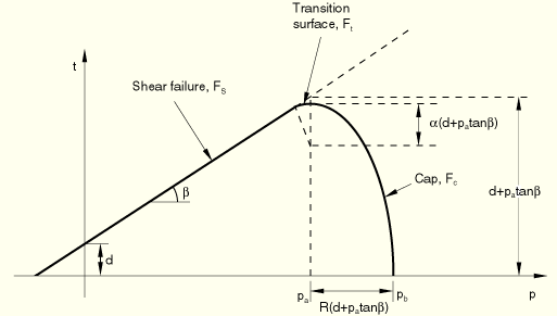
The yield surface has two principal segments: a pressure-dependent Drucker-Prager shear failure segment and a compression cap segment, as shown in Figure 18.3.2–1. The Drucker-Prager failure segment is a perfectly plastic yield surface (no hardening). Plastic flow on this segment produces inelastic volume increase (dilation) that causes the cap to soften. On the cap surface plastic flow causes the material to compact. The model is described in detail in “Drucker-Prager/Cap model for geological materials,” Section 4.4.4 of the ABAQUS Theory Manual.
The Drucker-Prager failure surface is written as
![]()
![]()
is the equivalent pressure stress,
![]()
is the Mises equivalent stress,
![]()
is the third stress invariant, and
![]()
is the deviatoric stress.
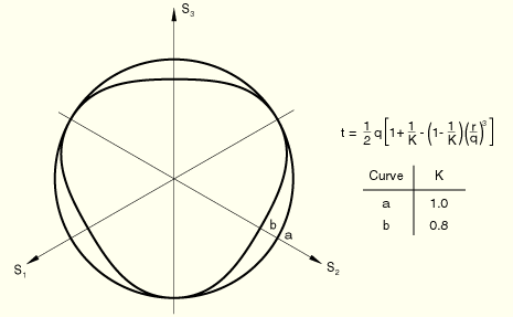
The cap yield surface has an elliptical shape with constant eccentricity in the meridional (p–t) plane (Figure 18.3.2–1) and also includes dependence on the third stress invariant in the deviatoric plane (Figure 18.3.2–2). The cap surface hardens or softens as a function of the volumetric inelastic strain: volumetric plastic and/or creep compaction (when yielding on the cap and/or creeping according to the consolidation mechanism, as described later in this section) causes hardening, while volumetric plastic and/or creep dilation (when yielding on the shear failure surface and/or creeping according to the cohesion mechanism, as described later in this section) causes softening. The cap yield surface is
![]()
![]()
The parameter ![]() is a small number (typically 0.01 to 0.05) used to define a transition yield surface,
is a small number (typically 0.01 to 0.05) used to define a transition yield surface,

You provide the variables d, ![]() , R,
, R, ![]() ,
, ![]() , and K to define the shape of the yield surface. In ABAQUS/Standard
, and K to define the shape of the yield surface. In ABAQUS/Standard ![]() , while in ABAQUS/Explicit K = 1 (
, while in ABAQUS/Explicit K = 1 (![]() ). If desired, combinations of these variables can also be defined as a tabular function of temperature and other predefined field variables.
). If desired, combinations of these variables can also be defined as a tabular function of temperature and other predefined field variables.
| Input File Usage: | *CAP PLASTICITY |
| ABAQUS/CAE Usage: | Property module: material editor: Mechanical |
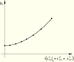
The hardening curve specified for this model interprets yielding in the hydrostatic pressure sense: the hydrostatic pressure yield stress is defined as a tabular function of the volumetric inelastic strain, and, if desired, a function of temperature and other predefined field variables. The range of values for which ![]() is defined should be sufficient to include all values of effective pressure stress that the material will be subjected to during the analysis.
is defined should be sufficient to include all values of effective pressure stress that the material will be subjected to during the analysis.
| Input File Usage: | *CAP HARDENING |
| ABAQUS/CAE Usage: | Property module: material editor: Mechanical |
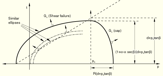
Plastic flow is defined by a flow potential that is associated in the deviatoric plane, associated in the cap region in the meridional plane, and nonassociated in the failure surface and transition regions in the meridional plane. The flow potential surface that we use in the meridional plane is shown in Figure 18.3.2–4: it is made up of an elliptical portion in the cap region that is identical to the cap yield surface,
Nonassociated flow implies that the material stiffness matrix is not symmetric and the unsymmetric matrix storage and solution scheme should be used in ABAQUS/Standard (see “Procedures: overview,” Section 6.1.1). If the region of the model in which nonassociated inelastic deformation is occurring is confined, it is possible that a symmetric approximation to the material stiffness matrix will give an acceptable rate of convergence; in such cases the unsymmetric matrix scheme may not be needed.
At least three experiments are required to calibrate the simplest version of the Cap model: a hydrostatic compression test (an oedometer test is also acceptable) and two uniaxial and/or triaxial compression tests (more than two tests are recommended for a more accurate calibration).
The hydrostatic compression test is performed by pressurizing the sample equally in all directions. The applied pressure and the volume change are recorded.
The uniaxial compression test involves compressing the sample between two rigid platens. The load and displacement in the direction of loading are recorded. The lateral displacements should also be recorded so that the correct volume changes can be calibrated.
Triaxial compression experiments are performed using a standard triaxial machine where a fixed confining pressure is maintained while the differential stress is applied. Several tests covering the range of confining pressures of interest are usually performed. Again, the stress and strain in the direction of loading are recorded, together with the lateral strain so that the correct volume changes can be calibrated.
Unloading measurements in these tests are useful to calibrate the elasticity, particularly in cases where the initial elastic region is not well defined.
The hydrostatic compression test stress-strain curve gives the evolution of the hydrostatic compression yield stress, ![]() , required for the cap hardening curve definition.
, required for the cap hardening curve definition.
The friction angle, ![]() , and cohesion, d, which define the shear failure dependence on hydrostatic pressure, are calculated by plotting the failure stresses of any two uniaxial and/or triaxial compression experiments in the pressure stress (p) versus shear stress (q) space: the slope of the straight line passing through the two points gives the angle
, and cohesion, d, which define the shear failure dependence on hydrostatic pressure, are calculated by plotting the failure stresses of any two uniaxial and/or triaxial compression experiments in the pressure stress (p) versus shear stress (q) space: the slope of the straight line passing through the two points gives the angle ![]() and the intersection with the q-axis gives d. For more details on the calibration of
and the intersection with the q-axis gives d. For more details on the calibration of ![]() and d, see the discussion on calibration in “Extended Drucker-Prager models,” Section 18.3.1.
and d, see the discussion on calibration in “Extended Drucker-Prager models,” Section 18.3.1.
R represents the curvature of the cap part of the yield surface and can be calibrated from a number of triaxial tests at high confining pressures (in the cap region). R must be between 0.0001 and 1000.0.
Classical “creep” behavior of materials that exhibit plasticity according to the capped Drucker-Prager plasticity model can be defined in ABAQUS/Standard. The creep behavior in such materials is intimately tied to the plasticity behavior (through the definitions of creep flow potentials and definitions of test data), so cap plasticity and cap hardening must be included in the material definition. If no rate-independent plastic behavior is desired in the model, large values for the cohesion, d, as well as large values for the compression yield stress, ![]() , should be provided in the plasticity definition: as a result the material follows the capped Drucker-Prager model while it creeps, without ever yielding. This capability is limited to cases in which there is no third stress invariant dependence of the yield surface (
, should be provided in the plasticity definition: as a result the material follows the capped Drucker-Prager model while it creeps, without ever yielding. This capability is limited to cases in which there is no third stress invariant dependence of the yield surface (![]() ) and cases in which the yield surface has no transition region (
) and cases in which the yield surface has no transition region (![]() ). The elastic behavior must be defined using linear isotropic elasticity (see “Defining isotropic elasticity” in “Linear elastic behavior,” Section 17.2.1).
). The elastic behavior must be defined using linear isotropic elasticity (see “Defining isotropic elasticity” in “Linear elastic behavior,” Section 17.2.1).
Creep behavior defined for the modified Drucker-Prager/Cap model is active only during soils consolidation, coupled temperature-displacement, and transient quasi-static procedures.
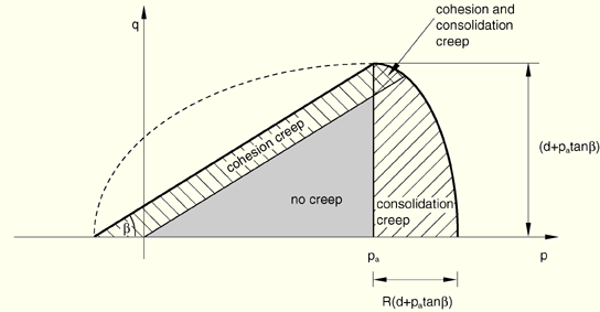
This model has two possible creep mechanisms that are active in different loading regions: one is a cohesion mechanism, which follows the type of plasticity active in the shear-failure plasticity region, and the other is a consolidation mechanism, which follows the type of plasticity active in the cap plasticity region. Figure 18.3.2–5 shows the regions of applicability of the creep mechanisms in p–q space.
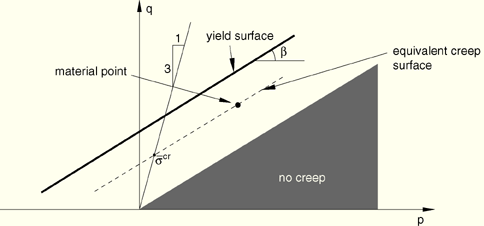
Consider the cohesion creep mechanism first. We adopt the notion of the existence of creep isosurfaces of stress points that share the same creep “intensity,” as measured by an equivalent creep stress. Since it is desirable to have the equivalent creep surface coincide with the yield surface, we define the equivalent creep surfaces by homogeneously scaling down the yield surface. In the p–q plane the equivalent creep surfaces translate into surfaces that are parallel to the yield surface, as depicted in Figure 18.3.2–6.
ABAQUS/Standard requires that cohesion creep properties be measured in a uniaxial compression test. The equivalent creep stress,![]()
Next, consider the consolidation creep mechanism. In this case we wish to make creep dependent on the hydrostatic pressure above a threshold value of ![]() , with a smooth transition to the areas in which the mechanism is not active (
, with a smooth transition to the areas in which the mechanism is not active (![]() ). Therefore, we define equivalent creep surfaces as constant hydrostatic pressure surfaces (vertical lines in the p–q plane). ABAQUS/Standard requires that consolidation creep properties be measured in a hydrostatic compression test. The effective creep pressure,
). Therefore, we define equivalent creep surfaces as constant hydrostatic pressure surfaces (vertical lines in the p–q plane). ABAQUS/Standard requires that consolidation creep properties be measured in a hydrostatic compression test. The effective creep pressure, ![]() , is then the point on the p-axis with a relative pressure of
, is then the point on the p-axis with a relative pressure of ![]() . This value is used in the uniaxial creep law. The equivalent volumetric creep strain rate produced by this type of law is defined as positive for a positive equivalent pressure. The internal tensor calculations in ABAQUS/Standard account for the fact that a positive pressure will produce negative (that is, compressive) volumetric creep components.
. This value is used in the uniaxial creep law. The equivalent volumetric creep strain rate produced by this type of law is defined as positive for a positive equivalent pressure. The internal tensor calculations in ABAQUS/Standard account for the fact that a positive pressure will produce negative (that is, compressive) volumetric creep components.
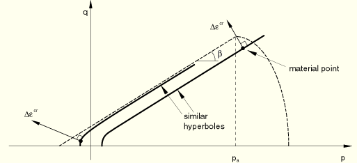
The creep strain rate produced by the cohesion mechanism is assumed to follow a potential that is similar to that of the creep strain rate in the Drucker-Prager creep model (“Extended Drucker-Prager models,” Section 18.3.1); that is, a hyperbolic function:
ABAQUS/Standard protects for numerical problems that may arise for very low stress values. See “Drucker-Prager/Cap model for geological materials,” Section 4.4.4 of the ABAQUS Theory Manual, for details.
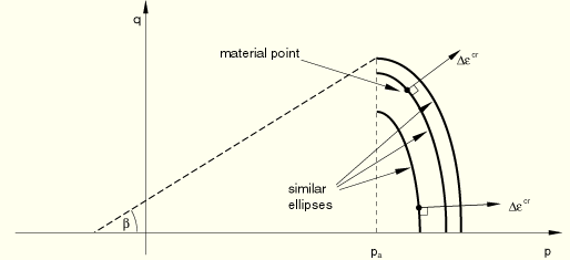
The creep strain rate produced by the consolidation mechanism is assumed to follow a potential that is similar to that of the plastic strain rate in the cap yield surface (Figure 18.3.2–8):
![]()
The consolidation creep potential is the von Mises circle in the deviatoric stress plane (the ![]() -plane). The volumetric components of creep strain from both mechanisms contribute to the hardening/softening of the cap, as described previously. For details on the behavior of these models refer to “Verification of creep integration,” Section 3.2.6 of the ABAQUS Benchmarks Manual.
-plane). The volumetric components of creep strain from both mechanisms contribute to the hardening/softening of the cap, as described previously. For details on the behavior of these models refer to “Verification of creep integration,” Section 3.2.6 of the ABAQUS Benchmarks Manual.
The use of a creep potential for the cohesion mechanism different from the equivalent creep surface implies that the material stiffness matrix is not symmetric, and the unsymmetric matrix storage and solution scheme should be used (see “Procedures: overview,” Section 6.1.1). If the region of the model in which cohesive inelastic deformation is occurring is confined, it is possible that a symmetric approximation to the material stiffness matrix will give an acceptable rate of convergence; in such cases the unsymmetric matrix scheme may not be needed.
The definition of the creep behavior is completed by specifying the equivalent “uniaxial behavior”—the creep “laws.” In many practical cases the creep laws are defined through user subroutine CREEP because creep laws are usually of complex form to fit experimental data. Data input methods are provided for some simple cases.
User subroutine CREEP provides a general capability for implementing viscoplastic models in which the strain rate potential can be written as a function of the equivalent stress and any number of “solution-dependent state variables.” When used in conjunction with these materials, the equivalent cohesion creep stress, ![]() , and the effective creep pressure,
, and the effective creep pressure, ![]() , are made available in the routine. Solution-dependent state variables are any variables that are used in conjunction with the constitutive definition and whose values evolve with the solution. Examples are hardening variables associated with the model. When a more general form is required for the stress potential, user subroutine UMAT can be used.
, are made available in the routine. Solution-dependent state variables are any variables that are used in conjunction with the constitutive definition and whose values evolve with the solution. Examples are hardening variables associated with the model. When a more general form is required for the stress potential, user subroutine UMAT can be used.
| Input File Usage: | Use either or both of the following options: |
*CAP CREEP, MECHANISM=COHESION, LAW=USER *CAP CREEP, MECHANISM=CONSOLIDATION, LAW=USER |
| ABAQUS/CAE Usage: | Define one or both of the following: |
Property module: material editor: Mechanical |
With respect to the cohesion mechanism, the power law is available
![]()
![]()
is the equivalent creep strain rate;
![]()
is the equivalent cohesion creep stress;
t
is the total time; and
A, n, and m
are user-defined creep material parameters specified as functions of temperature and field variables.
In using this form of the power law model with the consolidation mechanism, ![]() can be replaced by
can be replaced by ![]() , the effective creep pressure, in the above relation.
, the effective creep pressure, in the above relation.
| Input File Usage: | Use either or both of the following options: |
*CAP CREEP, MECHANISM=COHESION, LAW=TIME *CAP CREEP, MECHANISM=CONSOLIDATION, LAW=TIME |
| ABAQUS/CAE Usage: | Define one or both of the following: |
Property module: material editor: Mechanical |
As an alternative to the “time hardening” form of the power law, as defined above, the corresponding “strain hardening” form can be used. For the cohesion mechanism this law has the form
![]()
In using this form of the power law model with the consolidation mechanism, ![]() can be replaced by
can be replaced by ![]() , the effective creep pressure, in the above relation.
, the effective creep pressure, in the above relation.
For physically reasonable behavior A and n must be positive and ![]() .
.
| Input File Usage: | Use either or both of the following options: |
*CAP CREEP, MECHANISM=COHESION, LAW=STRAIN *CAP CREEP, MECHANISM=CONSOLIDATION, LAW=STRAIN |
| ABAQUS/CAE Usage: | Define one or both of the following: |
Property module: material editor: Mechanical |
A second cohesion creep law available as data input is a variation of the Singh-Mitchell law:
![]()
In using this variation of the Singh-Mitchell law with the consolidation mechanism, ![]() can be replaced by
can be replaced by ![]() , the effective creep pressure, in the above relation.
, the effective creep pressure, in the above relation.
| Input File Usage: | Use either or both of the following options: |
*CAP CREEP, MECHANISM=COHESION, LAW=SINGHM *CAP CREEP, MECHANISM=CONSOLIDATION, LAW=SINGHM |
| ABAQUS/CAE Usage: | Define one or both of the following: |
Property module: material editor: Mechanical |
Depending on the choice of units for the creep laws described above, the value of A may be very small for typical creep strain rates. If A is less than 10–27, numerical difficulties can cause errors in the material calculations; therefore, use another system of units to avoid such difficulties in the calculation of creep strain increments.
ABAQUS/Standard provides both explicit and implicit time integration of creep and swelling behavior. The choice of the time integration scheme depends on the procedure type, the parameters specified for the procedure, the presence of plasticity, and whether or not a geometric linear or nonlinear analysis is requested, as discussed in “Rate-dependent plasticity: creep and swelling,” Section 18.2.4.
The initial stress at a point can be defined (see “Defining initial stresses” in “Initial conditions,” Section 27.2.1). If such a stress point lies outside the initially defined cap or transition yield surfaces and under the projection of the shear failure surface in the p–t plane (illustrated in Figure 18.3.2–1), ABAQUS will try to adjust the initial position of the cap to make the stress point lie on the yield surface and a warning message will be issued. If the stress point lies outside the Drucker-Prager failure surface (or above its projection), an error message will be issued and execution will be terminated.
The modified Drucker-Prager/Cap material behavior can be used with plane strain, generalized plane strain, axisymmetric, and three-dimensional solid (continuum) elements. This model cannot be used with elements for which the assumed stress state is plane stress (plane stress, shell, and membrane elements).
In addition to the standard output identifiers available in ABAQUS (“ABAQUS/Standard output variable identifiers,” Section 4.2.1, and “ABAQUS/Explicit output variable identifiers,” Section 4.2.2), the following variables have special meaning in the cap plasticity/creep model:
PEEQ |
|
PEQC | All equivalent plastic strains, one for each of the yield/failure surfaces of the model. |
CEEQ | Equivalent creep strain produced by the cohesion creep mechanism, defined as |
CESW | Equivalent creep strain produced by the consolidation creep mechanism, defined as |