
Products: ABAQUS/Standard ABAQUS/CAE
The classical deviatoric metal creep behavior in ABAQUS/Standard:
can be defined using user subroutine CREEP or by providing parameters as input for some simple creep laws;
can model either isotropic creep (using Mises stress potential) or anisotropic creep (using Hill's anisotropic stress potential);
is active only during steps using the coupled temperature-displacement procedure, the transient soils consolidation procedure, and the quasi-static procedure;
requires that the material's elasticity be defined as linear elastic behavior;
can be modified to implement the auxiliary creep hardening rules specified in Nuclear Standard NEF 9-5T, “Guidelines and Procedures for Design of Class 1 Elevated Temperature Nuclear System Components”; these rules are exercised by means of a constitutive model developed by Oak Ridge National Laboratory (“ORNL – Oak Ridge National Laboratory constitutive model,” Section 18.2.12);
can be used in combination with creep strain rate control in analyses in which the creep strain rate must be kept within a certain range; and
can potentially result in errors in calculated creep strains if anisotropic creep and plasticity occur simultaneously (discussed below).
uses unidirectional creep as part of the model of the gasket's thickness-direction behavior;
can be defined using user subroutine CREEP or by providing parameters as input for some simple creep laws;
is active only during steps using the quasi-static procedure; and
requires that an elastic-plastic model be used to define the rate-independent part of the thickness-direction behavior of the gasket.
can be defined using user subroutine CREEP or by providing tabular input;
can be either isotropic or anisotropic;
is active only during steps using the coupled temperature-displacement procedure, the transient soils consolidation procedure, and the quasi-static procedure; and
requires that the material's elasticity be defined as linear elastic behavior.
Creep behavior is specified by the equivalent uniaxial behavior—the creep “law.” In practical cases creep laws are typically of very complex form to fit experimental data; therefore, the laws are defined with user subroutine CREEP, as discussed below. Alternatively, two common creep laws are provided in ABAQUS/Standard: the power law and the hyperbolic-sine law models. These standard creep laws are used for modeling secondary or steady-state creep. Creep is defined by including creep behavior in the material model definition (“Material data definition,” Section 16.1.2). Alternatively, creep can be defined in conjunction with gasket behavior to define the rate-dependent behavior of a gasket.
| Input File Usage: | Use the following options to include creep behavior in the material model definition: |
*MATERIAL
*CREEP
Use the following options to define creep in conjunction with gasket behavior: *GASKET BEHAVIOR *CREEP |
| ABAQUS/CAE Usage: | Property module: material editor: Mechanical |
The power-law creep model is attractive for its simplicity. However, it is limited in its range of application. The time-hardening version of the power-law creep model is most suitable when the stress state remains essentially constant. The strain-hardening version of power-law creep should be used when the stress state varies during an analysis. For either version of the power law, the stresses should be relatively low.
In regions of high stress, such as around a crack tip, the creep strain rates frequently show an exponential dependence of stress. The hyperbolic-sine creep law shows exponential dependence on the stress, ![]() , at high stress levels (
, at high stress levels (![]() , where
, where ![]() is the yield stress) and reduces to the power-law at low stress levels (with no explicit time dependence).
is the yield stress) and reduces to the power-law at low stress levels (with no explicit time dependence).
None of the above models is suitable for modeling creep under cyclic loading. The ORNL model (“ORNL – Oak Ridge National Laboratory constitutive model,” Section 18.2.12) is an empirical model for stainless steel that gives approximate results for cyclic loading without having to perform the cyclic loading numerically. Generally, creep models for cyclic loading are complicated and must be added to a model with user subroutine CREEP or with user subroutine UMAT.
If creep and plasticity occur simultaneously and implicit creep integration is in effect, both behaviors may interact and a coupled system of constitutive equations needs to be solved. If creep and plasticity are isotropic, ABAQUS/Standard properly takes into account such coupled behavior, even if the elasticity is anisotropic. However, if creep and plasticity are anisotropic, ABAQUS/Standard integrates the creep equations without taking plasticity into account, which may lead to substantial errors in the creep strains. This situation develops only if plasticity and creep are active at the same time, such as would occur during a long-term load increase; one would not expect to have a problem if there is a short-term preloading phase in which plasticity dominates, followed by a creeping phase in which no further yielding occurs. Integration of the creep laws and rate-dependent plasticity are discussed in “Rate-dependent metal plasticity (creep),” Section 4.3.4 of the ABAQUS Theory Manual.
The power-law model can be used in its “time hardening” form or in the corresponding “strain hardening” form.
The “time hardening” form is the simpler of the two forms of the power-law model:
![]()
![]()
is the uniaxial equivalent creep strain rate, ![]()
![]()
is the uniaxial equivalent deviatoric stress,
t
is the total time, and
A, n, and m
are defined by you as functions of temperature.
| Input File Usage: | *CREEP, LAW=TIME |
| ABAQUS/CAE Usage: | Property module: material editor: Mechanical |
The “strain hardening” form of the power law is
![]()
| Input File Usage: | *CREEP, LAW=STRAIN |
| ABAQUS/CAE Usage: | Property module: material editor: Mechanical |
Depending on the choice of units for either form of the power law, the value of A may be very small for typical creep strain rates. If A is less than 10–27, numerical difficulties can cause errors in the material calculations; therefore, use another system of units to avoid such difficulties in the calculation of creep strain increments.
The hyperbolic-sine law is available in the form
![]()
![]() and
and ![]()
are defined above,
![]()
is the temperature,
![]()
is the user-defined value of absolute zero on the temperature scale used,
![]()
is the activation energy,
R
is the universal gas constant, and
A, B, and n
are other material parameters.
| Input File Usage: | Use both of the following options: |
*CREEP, LAW=HYPERBOLIC *PHYSICAL CONSTANTS, ABSOLUTE ZERO= |
| ABAQUS/CAE Usage: | Define both of the following: |
Property module: material editor: Mechanical Any module: Model |
Anisotropic creep can be defined to specify the stress ratios that appear in Hill's function. You must define the ratios ![]() in each direction that will be used to scale the stress value when the creep strain rate is calculated. The ratios can be defined as constant or dependent on temperature and other predefined field variables. The ratios are defined with respect to the user-defined local material directions or the default directions (see “Orientations,” Section 2.2.5). Further details are provided in “Anisotropic yield/creep,” Section 18.2.6. Anisotropic creep is not available when creep is used to define a rate-dependent gasket behavior since only the gasket thickness-direction behavior can have rate-dependent behavior.
in each direction that will be used to scale the stress value when the creep strain rate is calculated. The ratios can be defined as constant or dependent on temperature and other predefined field variables. The ratios are defined with respect to the user-defined local material directions or the default directions (see “Orientations,” Section 2.2.5). Further details are provided in “Anisotropic yield/creep,” Section 18.2.6. Anisotropic creep is not available when creep is used to define a rate-dependent gasket behavior since only the gasket thickness-direction behavior can have rate-dependent behavior.
| Input File Usage: | *POTENTIAL |
| ABAQUS/CAE Usage: | Property module: material editor: Mechanical |
As with the creep laws, volumetric swelling laws are usually complex and are most conveniently specified in user subroutine CREEP as discussed below. However, a means of tabular input is also provided for the form
![]()
Volumetric swelling cannot be used to define a rate-dependent gasket behavior.
| Input File Usage: | *SWELLING |
| ABAQUS/CAE Usage: | Property module: material editor: Mechanical |
Anisotropy can easily be included in the swelling behavior. If anisotropic swelling behavior is defined, the swelling strain rate in each material direction is expressed as
![]()
| ABAQUS/CAE Usage: | Property module: material editor: Mechanical |
User subroutine CREEP provides a very general capability for implementing viscoplastic models such as creep and swelling models in which the strain rate potential can be written as a function of equivalent pressure stress, p; the Mises or Hill's equivalent deviatoric stress, ![]() ; and any number of solution-dependent state variables. Solution-dependent state variables are used in conjunction with the constitutive definition; their values evolve with the solution and can be defined in this subroutine. Examples are hardening variables associated with the model.
; and any number of solution-dependent state variables. Solution-dependent state variables are used in conjunction with the constitutive definition; their values evolve with the solution and can be defined in this subroutine. Examples are hardening variables associated with the model.
The user subroutine can also be used to define very general rate- and time-dependent thickness-direction gasket behavior. When an even more general form is required for the strain rate potential, user subroutine UMAT (“User-defined mechanical material behavior,” Section 20.8.1) can be used.
| ABAQUS/CAE Usage: | Use one or both of the following models. Only the first model can be used to define gasket behavior. |
Property module: material editor:
Mechanical |
You can specify that no creep (or viscoelastic) response can occur during certain analysis steps, even if creep (or viscoelastic) material properties have been defined.
| Input File Usage: | Use one of the following options: |
*COUPLED TEMPERATURE-DISPLACEMENT, CREEP=NONE *SOILS, CONSOLIDATION, CREEP=NONE |
| ABAQUS/CAE Usage: | Use one of the following options: |
Step module: Create Step: Coupled temp-displacement: toggle off Include creep/swelling/ viscoelastic behavior Soils: Pore fluid response: Transient consolidation: toggle off Include creep/swelling/viscoelastic behavior |
Explicit integration, implicit integration, or both integration schemes can be used in a creep analysis, depending on the procedure used, the parameters specified for the procedure, the presence of plasticity, and whether or not geometric nonlinearity is requested.
Nonlinear creep problems are often solved efficiently by forward-difference integration of the inelastic strains (the “initial strain” method). This explicit method is computationally efficient because, unlike implicit methods, iteration is not required. Although this method is only conditionally stable, the numerical stability limit of the explicit operator is usually sufficiently large to allow the solution to be developed in a small number of time increments.
ABAQUS/Standard uses either an explicit or an implicit integration scheme or switches from explicit to implicit in the same step. These schemes are outlined first, followed by a description of which procedures use these integration schemes.
Integration scheme 1: Starts with explicit integration and switches to implicit integration based on either stability or if plasticity is active. The stability limit used in explicit integration is discussed in the next section.
Integration scheme 2: Starts with explicit integration and switches to implicit integration when plasticity is active. The stability criterion does not play a role here.
Integration scheme 3: Always uses implicit integration.
The use of the above integration schemes is determined by the procedure type, your choice of the integration type to be used, as well as whether or not geometric nonlinearity is requested. For quasi-static and coupled temperature-displacement procedures, if you do not choose an integration type, integration scheme 1 is used for a geometrically linear analysis and integration scheme 3 is used for a geometrically nonlinear analysis. You can force ABAQUS/Standard to use explicit integration for creep and swelling effects in coupled temperature-displacement or quasi-static procedures, when plasticity is not active throughout the step (integration scheme 2). Explicit integration can be used regardless of whether or not geometric nonlinearity has been requested (see “General and linear perturbation procedures,” Section 6.1.2).
For a transient soils consolidation procedure, the implicit integration scheme (integration scheme 3) is always used, irrespective of whether a geometrically linear or nonlinear analysis is performed.
| Input File Usage: | Use one of the following options to restrict ABAQUS/Standard to using explicit integration: |
*VISCO, CREEP=EXPLICIT *COUPLED TEMPERATURE-DISPLACEMENT, CREEP=EXPLICIT |
| ABAQUS/CAE Usage: | Use one of the following options to restrict ABAQUS/Standard to using explicit integration: |
Step module: Create Step: Visco: Incrementation: Creep/swelling/viscoelastic integration: Explicit Coupled temp-displacement: toggle on Include creep/swelling/ viscoelastic behavior: Incrementation: Creep/swelling/viscoelastic integration: Explicit |
ABAQUS/Standard monitors the stability limit automatically during explicit integration. If, at any point in the model, the creep strain increment ![]() is larger than the total elastic strain, the problem will become unstable. Therefore, a stable time step,
is larger than the total elastic strain, the problem will become unstable. Therefore, a stable time step, ![]() , is calculated every increment by
, is calculated every increment by
![]()
![]()
![]()
![]()
is the gradient of the deviatoric stress potential,
![]()
is the elasticity matrix, and
![]()
is an effective elastic modulus—for isotropic elasticity ![]() can be approximated by Young's modulus.
can be approximated by Young's modulus.
At every increment for which explicit integration is performed, the stable time increment, ![]() , is compared to the critical time increment,
, is compared to the critical time increment, ![]() , which is calculated as follows:
, which is calculated as follows:
![]()
The integration tolerance must be chosen so that increments in stress, ![]() , are calculated accurately. Consider a one-dimensional example. The stress increment,
, are calculated accurately. Consider a one-dimensional example. The stress increment, ![]() , is
, is
![]()
![]()
![]()
![]()
![]()
| Input File Usage: | Use one of the following options: |
*VISCO, CETOL=errtol *COUPLED TEMPERATURE-DISPLACEMENT, CETOL=errtol *SOILS, CONSOLIDATION, CETOL=errtol |
| ABAQUS/CAE Usage: | Use one of the following options: |
Step module: Create Step: Visco: Incrementation: toggle on Creep/swelling/viscoelastic strain error tolerance, and enter a value Coupled temp-displacement: toggle on Include creep/swelling/ viscoelastic behavior: Incrementation: toggle on Creep/swelling/ viscoelastic strain error tolerance, and enter a value Soils: Pore fluid response: Transient consolidation: toggle on Include creep/swelling/viscoelastic behavior: Incrementation: toggle on Creep/swelling/viscoelastic strain error tolerance, and enter a value |
In superplastic forming a controllable pressure is applied to deform a body. Superplastic materials can deform to very large strains, provided that the strain rates of the deformation are maintained within very tight tolerances. The objective of the superplastic analysis is to predict how the pressure must be controlled to form the component as fast as possible without exceeding a superplastic strain rate anywhere in the material.
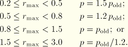
To achieve this using ABAQUS/Standard, the controlling algorithm is as follows. During an increment ABAQUS/Standard calculates ![]() , the maximum value of the ratio of the equivalent creep strain rate to the target creep strain rate for any integration point in a specified element set. If
, the maximum value of the ratio of the equivalent creep strain rate to the target creep strain rate for any integration point in a specified element set. If ![]() is less than 0.2 or greater than 3.0 in a given increment, the increment is abandoned and restarted with the following load modifications:
is less than 0.2 or greater than 3.0 in a given increment, the increment is abandoned and restarted with the following load modifications:
![]()
When you activate the above algorithm, the loading in a creep and/or swelling problem can be controlled on the basis of the maximum equivalent creep strain rate found in a defined element set. As a minimum requirement, this method is used to define a target equivalent creep strain rate; however, if required, it can also be used to define the target creep strain rate as a function of equivalent creep strain (measured as log strain), temperature, and other predefined field variables. The creep strain dependency curve at each temperature must always start at zero equivalent creep strain.
A solution-dependent amplitude is used to define the minimum and maximum limits of the loading (see “Defining a solution-dependent amplitude for superplastic forming analysis” in “Amplitude curves,” Section 27.1.2). Any number or combination of loads can be used. The current value of ![]() is available for output as discussed below.
is available for output as discussed below.
| Input File Usage: | Use all of the following options: |
*AMPLITUDE, NAME=name, DEFINITION=SOLUTION DEPENDENT
*CLOAD, *DLOAD, *DSLOAD, and/or *BOUNDARY with
AMPLITUDE=name
*CREEP STRAIN RATE CONTROL, AMPLITUDE=name, ELSET=elset
The *AMPLITUDE option must appear in the model definition portion of an input file, while the loading options (*CLOAD, *DLOAD, *DSLOAD, and *BOUNDARY) and the *CREEP STRAIN RATE CONTROL option should appear in each relevant step definition. |
| ABAQUS/CAE Usage: | Creep strain rate control is not supported in ABAQUS/CAE. |
Rate-dependent plasticity (creep and swelling behavior) can be used with any continuum, shell, membrane, gasket, and beam element in ABAQUS/Standard that has displacement degrees of freedom. Creep (but not swelling) can also be defined in the thickness direction of any gasket element in conjunction with the gasket behavior definition.
In addition to the standard output identifiers available in ABAQUS/Standard (“ABAQUS/Standard output variable identifiers,” Section 4.2.1), the following variables relate directly to creep and swelling models:
CEEQ | Equivalent creep strain, |
CESW | Magnitude of swelling strain. |
RATIO | Maximum value of the ratio of the equivalent creep strain rate to the target creep strain rate, |
AMPCU | Current value of the solution-dependent amplitude. |