Products: ABAQUS/Standard ABAQUS/Explicit ABAQUS/CAE
The extended Drucker-Prager models:
are used to model frictional materials, which are typically granular-like soils and rock, and exhibit pressure-dependent yield (the material becomes stronger as the pressure increases);
are used to model materials in which the compressive yield strength is greater than the tensile yield strength, such as those commonly found in composite and polymeric materials;
allow a material to harden and/or soften isotropically;
generally allow for volume change with inelastic behavior: the flow rule, defining the inelastic straining, allows simultaneous inelastic dilation (volume increase) and inelastic shearing;
can include creep in ABAQUS/Standard if the material exhibits long-term inelastic deformations;
can be defined to be sensitive to the rate of straining, as is often the case in polymeric materials;
can be used in conjunction with either the elastic material model (“Linear elastic behavior,” Section 17.2.1) or, in ABAQUS/Standard if creep is not defined, the porous elastic material model (“Elastic behavior of porous materials,” Section 17.3.1);
can be used in conjunction with the models of progressive damage and failure in ABAQUS/Explicit (“Damage and failure for ductile metals: overview,” Section 19.2.1) to specify different damage initiation criteria and damage evolution laws that allow for the progressive degradation of the material stiffness and the removal of elements from the mesh; and
are intended to simulate material response under essentially monotonic loading.
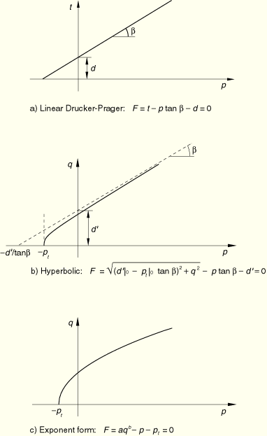
The yield criteria for this class of models are based on the shape of the yield surface in the meridional plane. In ABAQUS/Standard the yield surface can have a linear form, a hyperbolic form, or a general exponent form; in ABAQUS/Explicit only the linear form is available. These surfaces are illustrated in Figure 18.3.1–1.
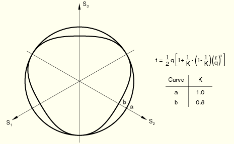
The stress invariants and other terms in each of the three related yield criteria are defined later in this section.The linear model (Figure 18.3.1–1a) provides for a possibly noncircular yield surface in the deviatoric plane (![]() -plane) to match different yield values in triaxial tension and compression, associated inelastic flow in the deviatoric plane, and separate dilation and friction angles. Input data parameters define the shape of the yield and flow surfaces in the meridional and deviatoric planes as well as other characteristics of inelastic behavior such that a range of simple theories is provided—the original Drucker-Prager model is available within this model. However, this model cannot provide a close match to Mohr-Coulomb behavior, as described later in this section.
-plane) to match different yield values in triaxial tension and compression, associated inelastic flow in the deviatoric plane, and separate dilation and friction angles. Input data parameters define the shape of the yield and flow surfaces in the meridional and deviatoric planes as well as other characteristics of inelastic behavior such that a range of simple theories is provided—the original Drucker-Prager model is available within this model. However, this model cannot provide a close match to Mohr-Coulomb behavior, as described later in this section.
The hyperbolic and general exponent models use a von Mises (circular) section in the deviatoric stress plane. In the meridional plane a hyperbolic flow potential is used for both models, which, in general, means nonassociated flow. These models are available only in ABAQUS/Standard.
The choice of model to be used depends largely on the analysis type, the kind of material, the experimental data available for calibration of the model parameters, and the range of pressure stress values that the material is likely to experience. It is common to have either triaxial test data at different levels of confining pressure or test data that are already calibrated in terms of a cohesion and a friction angle and, sometimes, a triaxial tensile strength value. If triaxial test data are available, the material parameters must be calibrated first. The accuracy with which the linear model can match these test data is limited by the fact that it assumes linear dependence of deviatoric stress on pressure stress. Although the hyperbolic model makes a similar assumption at high confining pressures, it provides a nonlinear relationship between deviatoric and pressure stress at low confining pressures, which may provide a better match of the triaxial experimental data. The hyperbolic model is useful for brittle materials for which both triaxial compression and triaxial tension data are available, which is a common situation for materials such as rocks. The most general of the three yield criteria is the exponent form. This criterion provides the most flexibility in matching triaxial test data. ABAQUS determines the material parameters required for this model directly from the triaxial test data. A least-squares fit that minimizes the relative error in stress is used for this purpose.
For cases where the experimental data are already calibrated in terms of a cohesion and a friction angle, the linear model can be used. If these parameters are provided for a Mohr-Coulomb model, it is necessary to convert them to Drucker-Prager parameters. The linear model is intended primarily for applications where the stresses are for the most part compressive. If tensile stresses are significant, hydrostatic tension data should be available (along with the cohesion and friction angle) and the hyperbolic model should be used.
Calibration of these models is discussed later in this section.
For granular materials these models are often used as a failure surface, in the sense that the material can exhibit unlimited flow when the stress reaches yield. This behavior is called perfect plasticity. The models are also provided with isotropic hardening. In this case plastic flow causes the yield surface to change size uniformly with respect to all stress directions. This hardening model is useful for cases involving gross plastic straining or in which the straining at each point is essentially in the same direction in strain space throughout the analysis. Although the model is referred to as an isotropic “hardening” model, strain softening, or hardening followed by softening, can be defined.
As strain rates increase, many materials show an increase in their yield strength. This effect becomes important in many polymers when the strain rates range between 0.1 and 1 per second; it can be very important for strain rates ranging between 10 and 100 per second, which are characteristic of high-energy dynamic events or manufacturing processes. The effect is generally not as important in granular materials. The evolution of the yield surface with plastic deformation is described in terms of the equivalent stress ![]() , which can be chosen as either the uniaxial compression yield stress, the uniaxial tension yield stress, or the shear (cohesion) yield stress:
, which can be chosen as either the uniaxial compression yield stress, the uniaxial tension yield stress, or the shear (cohesion) yield stress:
![]()
is the equivalent plastic strain rate, defined for the linear Drucker-Prager model as
![]()
=![]() if hardening is defined in uniaxial compression;
if hardening is defined in uniaxial compression;
![]()
=![]() if hardening is defined in uniaxial tension;
if hardening is defined in uniaxial tension;
![]()
=![]() if hardening is defined in pure shear,
if hardening is defined in pure shear,
![]()
![]()
is the equivalent plastic strain;
![]()
is temperature; and
![]()
are other predefined field variables.
The functional dependence ![]() includes hardening as well as rate-dependent effects. The material data can be input either directly in a tabular format or by correlating it to static relations based on yield stress ratios.
includes hardening as well as rate-dependent effects. The material data can be input either directly in a tabular format or by correlating it to static relations based on yield stress ratios.
Rate dependence as described here is most suitable for moderate- to high-speed events in ABAQUS/Standard. Time-dependent inelastic deformation at low deformation rates can be better represented by creep models. Such inelastic deformation, which can coexist with rate-independent plastic deformation, is described later in this section. However, the existence of creep in an ABAQUS/Standard material definition precludes the use of rate dependence as described here.
When using the Drucker-Prager material model, ABAQUS allows you to prescribe initial hardening by defining initial equivalent plastic strain values, as discussed below along with other details regarding the use of initial conditions.
Test data are entered as tables of yield stress values versus equivalent plastic strain at different equivalent plastic strain rates; one table per strain rate. Compression data are more commonly available for geological materials, whereas tension data are usually available for polymeric materials. The guidelines on how to enter these data are provided in “Rate-dependent yield,” Section 18.2.3.
| Input File Usage: | *DRUCKER PRAGER HARDENING, RATE= |
| ABAQUS/CAE Usage: | Property module: material editor: Mechanical |
Alternatively, the strain rate behavior can be assumed to be separable, so that the stress-strain dependence is similar—or, in ABAQUS/Explicit, identical—at all strain rates:
![]()
Two methods are offered to define R in ABAQUS: specifying an overstress power law or defining the variable R directly as a tabular function of ![]() .
.
The Cowper-Symonds overstress power law has the form
![]()
| Input File Usage: | Use both of the following options: |
*DRUCKER PRAGER HARDENING *RATE DEPENDENT, TYPE=POWER LAW |
| ABAQUS/CAE Usage: | Property module: material editor: Mechanical |
When R is entered directly, it is entered as a tabular function of the equivalent plastic strain rate, ![]() ; temperature,
; temperature, ![]() ; and predefined field variables,
; and predefined field variables, ![]() .
.
| Input File Usage: | Use both of the following options: |
*DRUCKER PRAGER HARDENING *RATE DEPENDENT, TYPE=YIELD RATIO |
| ABAQUS/CAE Usage: | Property module: material editor: Mechanical |
The yield stress surface makes use of two invariants, defined as the equivalent pressure stress,
![]()
![]()
![]()
![]()
The linear model is available in ABAQUS/Standard and ABAQUS/Explicit. The model is written in terms of all three stress invariants. It provides for a possibly noncircular yield surface in the deviatoric plane to match different yield values in triaxial tension and compression, associated inelastic flow in the deviatoric plane, and separate dilation and friction angles.
The linear Drucker-Prager criterion (see Figure 18.3.1–1a) is written as
![]()
![]()
is the slope of the linear yield surface in the p–t stress plane and is commonly referred to as the friction angle of the material;
d
is the cohesion of the material; and
![]()
is the ratio of the yield stress in triaxial tension to the yield stress in triaxial compression and, thus, controls the dependence of the yield surface on the value of the intermediate principal stress (see Figure 18.3.1–2).
In the case of hardening defined in uniaxial compression, the linear yield criterion precludes friction angles ![]() 71.5° (
71.5° (![]() 3), which is unlikely to be a limitation for real materials.
3), which is unlikely to be a limitation for real materials.
When ![]() ,
, ![]() , which implies that the yield surface is the von Mises circle in the deviatoric principal stress plane (the
, which implies that the yield surface is the von Mises circle in the deviatoric principal stress plane (the ![]() -plane), in which case the yield stresses in triaxial tension and compression are the same. To ensure that the yield surface remains convex requires
-plane), in which case the yield stresses in triaxial tension and compression are the same. To ensure that the yield surface remains convex requires ![]() .
.
The cohesion, d, of the material is related to the input data as
G is the flow potential, chosen in this model as
![]()
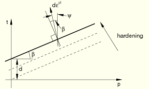
For granular materials the linear model is normally used with nonassociated flow in the p–t plane, in the sense that the flow is assumed to be normal to the yield surface in the ![]() -plane but at an angle
-plane but at an angle ![]() to the t-axis in the p–t plane, where usually
to the t-axis in the p–t plane, where usually ![]() , as illustrated in Figure 18.3.1–3. Associated flow results from setting
, as illustrated in Figure 18.3.1–3. Associated flow results from setting ![]() . The original Drucker-Prager model is available by setting
. The original Drucker-Prager model is available by setting ![]() and
and ![]() . Nonassociated flow is also generally assumed when the model is used for polymeric materials. If
. Nonassociated flow is also generally assumed when the model is used for polymeric materials. If ![]() , the inelastic deformation is incompressible; if
, the inelastic deformation is incompressible; if ![]() , the material dilates. Hence,
, the material dilates. Hence, ![]() is referred to as the dilation angle.
is referred to as the dilation angle.
The relationship between the flow potential and the incremental plastic strain for the linear model is discussed in detail in “Models for granular or polymer behavior,” Section 4.4.2 of the ABAQUS Theory Manual.
| Input File Usage: | *DRUCKER PRAGER, SHEAR CRITERION=LINEAR |
| ABAQUS/CAE Usage: | Property module: material editor: Mechanical |
Nonassociated flow implies that the material stiffness matrix is not symmetric; therefore, the unsymmetric matrix storage and solution scheme should be used in ABAQUS/Standard (see “Procedures: overview,” Section 6.1.1). If the difference between ![]() and
and ![]() is not large and the region of the model in which inelastic deformation is occurring is confined, it is possible that a symmetric approximation to the material stiffness matrix will give an acceptable rate of convergence and the unsymmetric matrix scheme may not be needed.
is not large and the region of the model in which inelastic deformation is occurring is confined, it is possible that a symmetric approximation to the material stiffness matrix will give an acceptable rate of convergence and the unsymmetric matrix scheme may not be needed.
In ABAQUS/Explicit the linear Drucker-Prager model can be used in conjunction with the models of progressive damage and failure discussed in “Damage and failure for ductile metals: overview,” Section 19.2.1. The capability allows for the specification of one or more damage initiation criteria, including ductile, shear, forming limit diagram (FLD), forming limit stress diagram (FLSD), and Müschenborn-Sonne forming limit diagram (MSFLD) criteria. After damage initiation, the material stiffness is degraded progressively according to the specified damage evolution response. The model offers two failure choices, including the removal of elements from the mesh as a result of tearing or ripping of the structure. The progressive damage models allow for a smooth degradation of the material stiffness, making them suitable for both quasi-static and dynamic situations.
| Input File Usage: | Use the following options: |
*PLASTIC *DAMAGE INITIATION *DAMAGE EVOLUTION |
| ABAQUS/CAE Usage: | Property module: material editor: Mechanical |
The hyperbolic and general exponent models available in ABAQUS/Standard are written in terms of the first two stress invariants only.
The hyperbolic yield criterion is a continuous combination of the maximum tensile stress condition of Rankine (tensile cut-off) and the linear Drucker-Prager condition at high confining stress. It is written as
![]()
![]()
is the initial hydrostatic tension strength of the material;
![]()
is the hardening parameter;
![]()
is the initial value of ![]() ; and
; and
![]()
is the friction angle measured at high confining pressure, as shown in Figure 18.3.1–1(b).
| Input File Usage: | *DRUCKER PRAGER, SHEAR CRITERION=HYPERBOLIC |
| ABAQUS/CAE Usage: | Property module: material editor: Mechanical |
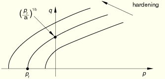
The general exponent form provides the most general yield criterion available in this class of models. The yield function is written as
![]()
![]() and
and ![]()
are material parameters that are independent of plastic deformation; and
![]()
is the hardening parameter that represents the hydrostatic tension strength of the material as shown in Figure 18.3.1–1(c).
| Input File Usage: | *DRUCKER PRAGER, SHEAR CRITERION=EXPONENT FORM |
| ABAQUS/CAE Usage: | Property module: material editor: Mechanical |
G is the flow potential, chosen in these models as a hyperbolic function:
![]()
![]()
is the dilation angle measured in the p–q plane at high confining pressure;
![]()
is the initial yield stress, taken from the user-specified Drucker-Prager hardening data; and
![]()
is a parameter, referred to as the eccentricity, that defines the rate at which the function approaches the asymptote (the flow potential tends to a straight line as the eccentricity tends to zero).
This flow potential, which is continuous and smooth, ensures that the flow direction is always uniquely defined. The function approaches the linear Drucker-Prager flow potential asymptotically at high confining pressure stress and intersects the hydrostatic pressure axis at 90°. A family of hyperbolic potentials in the meridional stress plane is shown in Figure 18.3.1–6. The flow potential is the von Mises circle in the deviatoric stress plane (the ![]() -plane).
-plane).
For the general exponent model flow is always nonassociated in the p–q plane. The default flow potential eccentricity is ![]() , which implies that the material has almost the same dilation angle over a wide range of confining pressure stress values. Increasing the value of
, which implies that the material has almost the same dilation angle over a wide range of confining pressure stress values. Increasing the value of ![]() provides more curvature to the flow potential, implying that the dilation angle increases more rapidly as the confining pressure decreases. Values of
provides more curvature to the flow potential, implying that the dilation angle increases more rapidly as the confining pressure decreases. Values of ![]() that are significantly less than the default value may lead to convergence problems if the material is subjected to low confining pressures because of the very tight curvature of the flow potential locally where it intersects the p-axis.
that are significantly less than the default value may lead to convergence problems if the material is subjected to low confining pressures because of the very tight curvature of the flow potential locally where it intersects the p-axis.
The relationship between the flow potential and the incremental plastic strain for the hyperbolic and general exponent models is discussed in detail in “Models for granular or polymer behavior,” Section 4.4.2 of the ABAQUS Theory Manual.
Nonassociated flow implies that the material stiffness matrix is not symmetric; therefore, the unsymmetric matrix storage and solution scheme should be used in ABAQUS/Standard (see “Procedures: overview,” Section 6.1.1). If the difference between ![]() and
and ![]() in the hyperbolic model is not large and if the region of the model in which inelastic deformation is occurring is confined, it is possible that a symmetric approximation to the material stiffness matrix will give an acceptable rate of convergence. In such cases the unsymmetric matrix scheme may not be needed.
in the hyperbolic model is not large and if the region of the model in which inelastic deformation is occurring is confined, it is possible that a symmetric approximation to the material stiffness matrix will give an acceptable rate of convergence. In such cases the unsymmetric matrix scheme may not be needed.
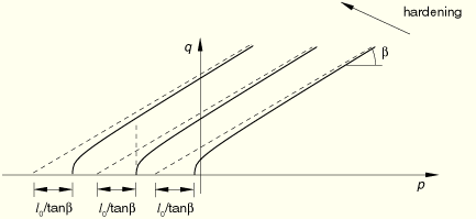
Data for geological materials are most commonly available from triaxial testing. In such a test the specimen is confined by a pressure stress that is held constant during the test. The loading is an additional tension or compression stress applied in one direction. Typical results include stress-strain curves at different levels of confinement, as shown in Figure 18.3.1–7.
Figure 18.3.1–7 Triaxial tests with stress-strain curves for typical geological materials at different levels of confinement.
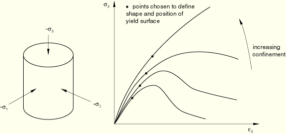
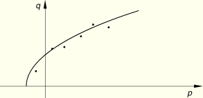
One stress data point from each stress-strain curve at a different level of confinement is plotted in the meridional stress plane (p–t plane if the linear model is to be used, or p–q plane if the hyperbolic or general exponent model will be used). This technique calibrates the shape and position of the yield surface, as shown in Figure 18.3.1–8, and is adequate to define a model if it is to be used as a failure surface (perfect plasticity).
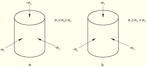
The models are also available with isotropic hardening, in which case hardening data are required to complete the calibration. In an isotropic hardening model plastic flow causes the yield surface to change size uniformly; in other words, only one of the stress-strain curves depicted in Figure 18.3.1–7 can be used to represent hardening. The curve that represents hardening most accurately over the range of loading conditions anticipated should be selected (usually the curve for the average anticipated value of pressure stress).As stated earlier, two types of triaxial test data are commonly available for geological materials. In a triaxial compression test the specimen is confined by pressure and an additional compression stress is superposed in one direction. Thus, the principal stresses are all negative, with ![]() (Figure 18.3.1–9a). In the preceding inequality
(Figure 18.3.1–9a). In the preceding inequality ![]() ,
, ![]() , and
, and ![]() are the maximum, intermediate, and minimum principal stresses, respectively.
are the maximum, intermediate, and minimum principal stresses, respectively.
The values of the stress invariants are
![]()
![]()
![]()
![]()
Fitting the best straight line through the triaxial compression results provides ![]() and d for the linear Drucker-Prager model.
and d for the linear Drucker-Prager model.
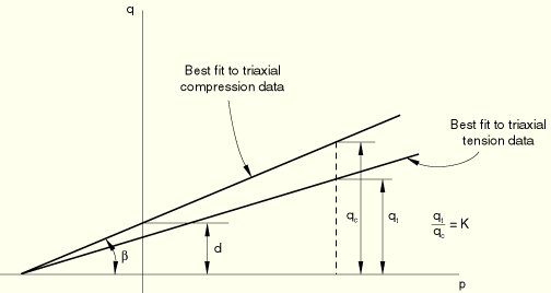
Triaxial tension data are also needed to define K in the linear Drucker-Prager model. Under triaxial tension the specimen is again confined by pressure, after which the pressure in one direction is reduced. In this case the principal stresses are ![]() (Figure 18.3.1–9b).
(Figure 18.3.1–9b).
The stress invariants are now
![]()
![]()
![]()
![]()
Thus, K can be found by plotting these test results as q versus p and again fitting the best straight line. The triaxial compression and tension lines must intercept the p-axis at the same point, and the ratio of values of q for triaxial tension and compression at the same value of p then gives K (Figure 18.3.1–10).
Fitting the best straight line through the triaxial compression results at high confining pressures provides ![]() and
and ![]() for the hyperbolic model. This fit is performed in the same manner as that used to obtain
for the hyperbolic model. This fit is performed in the same manner as that used to obtain ![]() and d for the linear Drucker-Prager model. In addition, hydrostatic tension data are required to complete the calibration of the hyperbolic model so that the initial hydrostatic tension strength,
and d for the linear Drucker-Prager model. In addition, hydrostatic tension data are required to complete the calibration of the hyperbolic model so that the initial hydrostatic tension strength, ![]() , can be defined.
, can be defined.
Given triaxial data in the meridional plane, ABAQUS/Standard provides a capability to determine the material parameters a, b, and ![]() required for the exponent model. The parameters are determined on the basis of a “best fit” of the triaxial test data at different levels of confining stress. A least-squares fit which minimizes the relative error in stress is used to obtain the “best fit” values for a, b, and
required for the exponent model. The parameters are determined on the basis of a “best fit” of the triaxial test data at different levels of confining stress. A least-squares fit which minimizes the relative error in stress is used to obtain the “best fit” values for a, b, and ![]() . The capability allows all three parameters to be calibrated or, if some of the parameters are known, only the remaining parameters to be calibrated. This ability is useful if only a few data points are available, in which case you may wish to fit the best straight line (
. The capability allows all three parameters to be calibrated or, if some of the parameters are known, only the remaining parameters to be calibrated. This ability is useful if only a few data points are available, in which case you may wish to fit the best straight line (![]() ) through the data points (effectively reducing the model to a linear Drucker-Prager model). Partial calibration can also be useful in a case when triaxial test data at low confinement are unreliable or unavailable, as is often the case for cohesionless materials. In this case a better fit may be obtained if the value of
) through the data points (effectively reducing the model to a linear Drucker-Prager model). Partial calibration can also be useful in a case when triaxial test data at low confinement are unreliable or unavailable, as is often the case for cohesionless materials. In this case a better fit may be obtained if the value of ![]() is specified and only a and b are calibrated.
is specified and only a and b are calibrated.
The data must be provided in terms of the principal stresses ![]() and
and ![]() , where
, where ![]() is the confining stress and
is the confining stress and ![]() is the stress in the loading direction. The ABAQUS sign convention must be followed such that tensile stresses are positive and compressive stresses are negative. One pair of stresses must be entered from each triaxial test. As many data points as desired can be entered from triaxial tests at different levels of confining stress.
is the stress in the loading direction. The ABAQUS sign convention must be followed such that tensile stresses are positive and compressive stresses are negative. One pair of stresses must be entered from each triaxial test. As many data points as desired can be entered from triaxial tests at different levels of confining stress.
If the exponent model is used as a failure surface (perfect plasticity), the Drucker-Prager hardening behavior does not have to be specified. The hydrostatic tension strength, ![]() , obtained from the calibration will then be used as the failure stress. However, if the Drucker-Prager hardening behavior is specified together with the triaxial test data, the value of
, obtained from the calibration will then be used as the failure stress. However, if the Drucker-Prager hardening behavior is specified together with the triaxial test data, the value of ![]() obtained from the calibration will be ignored. In this case ABAQUS/Standard will interpolate
obtained from the calibration will be ignored. In this case ABAQUS/Standard will interpolate ![]() directly from the hardening data.
directly from the hardening data.
| Input File Usage: | Use both of the following options: |
*DRUCKER PRAGER, SHEAR CRITERION=EXPONENT FORM, TEST DATA *TRIAXIAL TEST DATA |
| ABAQUS/CAE Usage: | Property module: material editor: Mechanical |
Sometimes experimental data are not directly available. Instead, you are provided with the friction angle and cohesion values for the Mohr-Coulomb model. In that case the simplest way to proceed in ABAQUS/Standard is to use the Mohr-Coulomb model (see “Mohr-Coulomb plasticity,” Section 18.3.3). In some situations it may be necessary to use the Drucker-Prager model instead of the Mohr-Coulomb model (such as when rate effects need to be considered), in which case we need to calculate values for the parameters of a Drucker-Prager model to provide a reasonable match to the Mohr-Coulomb parameters.
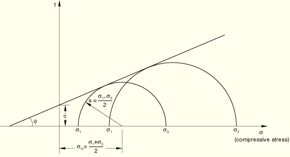
The Mohr-Coulomb failure model is based on plotting Mohr's circle for states of stress at failure in the plane of the maximum and minimum principal stresses. The failure line is the best straight line that touches these Mohr's circles (Figure 18.3.1–11).
Therefore, the Mohr-Coulomb model is defined by
![]()
![]()
Substituting for ![]() and
and ![]() , multiplying both sides by
, multiplying both sides by ![]() , and reducing, the Mohr-Coulomb model can be written as
, and reducing, the Mohr-Coulomb model can be written as
![]()
![]()
![]()
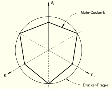
The Mohr-Coulomb model assumes that failure is independent of the value of the intermediate principal stress, but the Drucker-Prager model does not. The failure of typical geotechnical materials generally includes some small dependence on the intermediate principal stress, but the Mohr-Coulomb model is generally considered to be sufficiently accurate for most applications. This model has vertices in the deviatoric plane (see Figure 18.3.1–12).
The implication is that, whenever the stress state has two equal principal stress values, the flow direction can change significantly with little or no change in stress. None of the models currently available in ABAQUS can provide such behavior; even in the Mohr-Coulomb model the flow potential is smooth. This limitation is generally not a key concern in many design calculations involving Coulomb-like materials, but it can limit the accuracy of the calculations, especially in cases where flow localization is important.
Plane strain problems are often encountered in geotechnical analysis; for example, long tunnels, footings, and embankments. Therefore, the constitutive model parameters are often matched to provide the same flow and failure response in plane strain.
The matching procedure described below is carried out in terms of the linear Drucker-Prager model but is also applicable to the hyperbolic model at high levels of confining stress.
The linear Drucker-Prager flow potential defines the plastic strain increment as
![]()
![]()
![]()
![]()
![]()
![]()
![]()
The Mohr-Coulomb yield surface in the ![]() plane is
plane is
![]()
![]()
![]()
These relationships provide a match between the Mohr-Coulomb material parameters and linear Drucker-Prager material parameters in plane strain. Consider the two extreme cases of flow definition: associated flow, ![]() , and nondilatant flow, when
, and nondilatant flow, when ![]() . For associated flow
. For associated flow
![]()
![]()
The difference between these two approaches increases with the friction angle; however, the results are not very different for typical friction angles, as illustrated in Table 18.3.1–1.
Table 18.3.1–1 Plane strain matching of Drucker-Prager and Mohr-Coulomb models.
| Mohr-Coulomb friction angle, | Associated flow | Nondilatant flow | ||
|---|---|---|---|---|
| Drucker-Prager friction angle, | Drucker-Prager friction angle, | |||
| 10° | 16.7° | 1.70 | 16.7° | 1.70 |
| 20° | 30.2° | 1.60 | 30.6° | 1.63 |
| 30° | 39.8° | 1.44 | 40.9° | 1.50 |
| 40° | 46.2° | 1.24 | 48.1° | 1.33 |
| 50° | 50.5° | 1.02 | 53.0° | 1.11 |
“Limit load calculations with granular materials,” Section 1.14.4 of the ABAQUS Benchmarks Manual, and “Finite deformation of an elastic-plastic granular material,” Section 1.14.5 of the ABAQUS Benchmarks Manual, show a comparison of the response of a simple loading of a granular material using the Drucker-Prager and Mohr-Coulomb models, using the plane strain approach to match the parameters of the two models.
Another approach to matching Mohr-Coulomb and Drucker-Prager model parameters for materials with low friction angles is to make the two models provide the same failure definition in triaxial compression and tension. The following matching procedure is applicable only to the linear Drucker-Prager model since this is the only model in this class that allows for different yield values in triaxial compression and tension.
We can rewrite the Mohr-Coulomb model in terms of principal stresses:
![]()
![]()
![]()
We wish to make these expressions identical to the Mohr-Coulomb model for all values of ![]() . This is possible by setting
. This is possible by setting
![]()
By comparing the Mohr-Coulomb model with the linear Drucker-Prager model,
![]()
![]()
![]()
These results for ![]() and
and ![]() provide linear Drucker-Prager parameters that match the Mohr-Coulomb model in triaxial compression and tension.
provide linear Drucker-Prager parameters that match the Mohr-Coulomb model in triaxial compression and tension.
The value of K in the linear Drucker-Prager model is restricted to ![]() for the yield surface to remain convex. The result for K shows that this implies
for the yield surface to remain convex. The result for K shows that this implies ![]() . Many real materials have a larger Mohr-Coulomb friction angle than this value. One approach in such circumstances is to choose
. Many real materials have a larger Mohr-Coulomb friction angle than this value. One approach in such circumstances is to choose ![]() and then to use the remaining equations to define
and then to use the remaining equations to define ![]() and
and ![]() . This approach matches the models for triaxial compression only, while providing the closest approximation that the model can provide to failure being independent of the intermediate principal stress. If
. This approach matches the models for triaxial compression only, while providing the closest approximation that the model can provide to failure being independent of the intermediate principal stress. If ![]() is significantly larger than 22°, this approach may provide a poor Drucker-Prager match of the Mohr-Coulomb parameters. Therefore, this matching procedure is not generally recommended; in ABAQUS/Standard use the Mohr-Coulomb model instead.
is significantly larger than 22°, this approach may provide a poor Drucker-Prager match of the Mohr-Coulomb parameters. Therefore, this matching procedure is not generally recommended; in ABAQUS/Standard use the Mohr-Coulomb model instead.
While using one-element tests to verify the calibration of the model, it should be noted that the ABAQUS output variables SP1, SP2, and SP3 correspond to the principal stresses ![]() ,
, ![]() , and
, and ![]() , respectively.
, respectively.
Classical “creep” behavior of materials that exhibit plasticity according to the extended Drucker-Prager models can be defined in ABAQUS/Standard. The creep behavior in such materials is intimately tied to the plasticity behavior (through the definitions of creep flow potentials and definitions of test data), so Drucker-Prager plasticity and Drucker-Prager hardening must be included in the material definition.
Creep and plasticity can be active simultaneously, in which case the resulting equations are solved in a coupled manner. To model creep only (without rate-independent plastic deformation), large values for the yield stress should be provided in the Drucker-Prager hardening definition: the result is that the material follows the Drucker-Prager model while it creeps, without ever yielding. When using this technique, a value must also be defined for the eccentricity, since, as described below, both the initial yield stress and eccentricity affect the creep potentials. This capability is limited to the linear model with a von Mises (circular) section in the deviatoric stress plane (![]() ; i.e., no third stress invariant effects are taken into account) and can be combined only with linear elasticity.
; i.e., no third stress invariant effects are taken into account) and can be combined only with linear elasticity.
Creep behavior defined by the extended Drucker-Prager model is active only during soils consolidation, coupled temperature-displacement, and transient quasi-static procedures.
The creep potential is hyperbolic, similar to the plastic flow potentials used in the hyperbolic and general exponent plasticity models. If creep properties are defined in ABAQUS/Standard, the linear Drucker-Prager plasticity model also uses a hyperbolic plastic flow potential. As a consequence, if two analyses are run, one in which creep is not activated and another in which creep properties are specified but produce virtually no creep flow, the plasticity solutions will not be exactly the same: the solution with creep not activated uses a linear plastic potential, whereas the solution with creep activated uses a hyperbolic plastic potential.
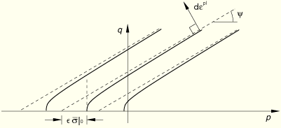
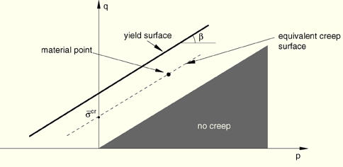
We adopt the notion of the existence of creep isosurfaces of stress points that share the same creep “intensity,” as measured by an equivalent creep stress. When the material plastifies, it is desirable to have the equivalent creep surface coincide with the yield surface; therefore, we define the equivalent creep surfaces by homogeneously scaling down the yield surface. In the p–q plane that translates into parallels to the yield surface, as depicted in Figure 18.3.1–13.
ABAQUS/Standard requires that creep properties be described in terms of the same type of data used to define work hardening properties. The equivalent creep stress,
Figure 18.3.1–13 shows how the equivalent point is determined when the material properties are in shear, with stress d. A consequence of these concepts is that there is a cone in p–q space inside which creep is not active since any point inside this cone would have a negative equivalent creep stress.
The creep strain rate in ABAQUS/Standard is assumed to follow from the same hyperbolic potential as the plastic strain rate (see Figure 18.3.1–6):
![]()
![]()
is the dilation angle measured in the p–q plane at high confining pressure;
![]()
is the initial yield stress taken from the user-specified Drucker-Prager hardening data; and
![]()
is a parameter, referred to as the eccentricity, that defines the rate at which the function approaches the asymptote (the creep potential tends to a straight line as the eccentricity tends to zero).
The default creep potential eccentricity is ![]() , which implies that the material has almost the same dilation angle over a wide range of confining pressure stress values. Increasing the value of
, which implies that the material has almost the same dilation angle over a wide range of confining pressure stress values. Increasing the value of ![]() provides more curvature to the creep potential, implying that the dilation angle increases as the confining pressure decreases. Values of
provides more curvature to the creep potential, implying that the dilation angle increases as the confining pressure decreases. Values of ![]() that are significantly less than the default value may lead to convergence problems if the material is subjected to low confining pressures, because of the very tight curvature of the creep potential locally where it intersects the p-axis. For details on the behavior of these models refer to “Verification of creep integration,” Section 3.2.6 of the ABAQUS Benchmarks Manual.
that are significantly less than the default value may lead to convergence problems if the material is subjected to low confining pressures, because of the very tight curvature of the creep potential locally where it intersects the p-axis. For details on the behavior of these models refer to “Verification of creep integration,” Section 3.2.6 of the ABAQUS Benchmarks Manual.
If the creep material properties are defined by a compression test, numerical problems may arise for very low stress values. ABAQUS/Standard protects for such a case, as described in “Models for granular or polymer behavior,” Section 4.4.2 of the ABAQUS Theory Manual.
The use of a creep potential different from the equivalent creep surface implies that the material stiffness matrix is not symmetric; therefore, the unsymmetric matrix storage and solution scheme should be used (see “Procedures: overview,” Section 6.1.1). If the difference between ![]() and
and ![]() is not large and the region of the model in which inelastic deformation is occurring is confined, it is possible that a symmetric approximation to the material stiffness matrix will give an acceptable rate of convergence and the unsymmetric matrix scheme may not be needed.
is not large and the region of the model in which inelastic deformation is occurring is confined, it is possible that a symmetric approximation to the material stiffness matrix will give an acceptable rate of convergence and the unsymmetric matrix scheme may not be needed.
The definition of creep behavior in ABAQUS/Standard is completed by specifying the equivalent “uniaxial behavior”—the creep “law.” In many practical cases the creep “law” is defined through user subroutine CREEP because creep laws are usually of very complex form to fit experimental data. Data input methods are provided for some simple cases, including two forms of a power law model and a variation of the Singh-Mitchell law.
User subroutine CREEP provides a very general capability for implementing viscoplastic models in ABAQUS/Standard in which the strain rate potential can be written as a function of the equivalent stress and any number of “solution-dependent state variables.” When used in conjunction with these material models, the equivalent creep stress, ![]() , is made available in the routine. Solution-dependent state variables are any variables that are used in conjunction with the constitutive definition and whose values evolve with the solution. Examples are hardening variables associated with the model. When a more general form is required for the stress potential, user subroutine UMAT can be used.
, is made available in the routine. Solution-dependent state variables are any variables that are used in conjunction with the constitutive definition and whose values evolve with the solution. Examples are hardening variables associated with the model. When a more general form is required for the stress potential, user subroutine UMAT can be used.
| Input File Usage: | *DRUCKER PRAGER CREEP, LAW=USER |
| ABAQUS/CAE Usage: | Property module: material editor: Mechanical |
The “time hardening” form of the power law model is
![]()
![]()
is the equivalent creep strain rate, defined so that ![]() if the equivalent creep stress is defined in uniaxial compression,
if the equivalent creep stress is defined in uniaxial compression, ![]() if defined in uniaxial tension, and
if defined in uniaxial tension, and ![]() if defined in pure shear, where
if defined in pure shear, where ![]() is the engineering shear creep strain;
is the engineering shear creep strain;
![]()
is the equivalent creep stress;
t
is the total time; and
A, n, and m
are user-defined creep material parameters specified as functions of temperature and field variables.
| Input File Usage: | *DRUCKER PRAGER CREEP, LAW=TIME |
| ABAQUS/CAE Usage: | Property module: material editor: Mechanical |
As an alternative to the “time hardening” form of the power law, as defined above, the corresponding “strain hardening” form can be used:
![]()
| Input File Usage: | *DRUCKER PRAGER CREEP, LAW=STRAIN |
| ABAQUS/CAE Usage: | Property module: material editor: Mechanical |
A second creep law available as data input is a variation of the Singh-Mitchell law:
![]()
| Input File Usage: | *DRUCKER PRAGER CREEP, LAW=SINGHM |
| ABAQUS/CAE Usage: | Property module: material editor: Mechanical |
Depending on the choice of units for the creep laws described above, the value of A may be very small for typical creep strain rates. If A is less than ![]() , numerical difficulties can cause errors in the material calculations; therefore, use another system of units to avoid such difficulties in the calculation of creep strain increments.
, numerical difficulties can cause errors in the material calculations; therefore, use another system of units to avoid such difficulties in the calculation of creep strain increments.
ABAQUS/Standard provides both explicit and implicit time integration of creep and swelling behavior. The choice of the time integration scheme depends on the procedure type, the parameters specified for the procedure, the presence of plasticity, and whether or not a geometric linear or nonlinear analysis is requested, as discussed in “Rate-dependent plasticity: creep and swelling,” Section 18.2.4.
There are cases when we need to study the behavior of a material that has already been subjected to some work hardening. For such cases ABAQUS allows you to prescribe initial conditions for the equivalent plastic strain, ![]() , by specifying the conditions directly (see “Initial conditions,” Section 27.2.1). For more complicated cases initial conditions can be defined in ABAQUS/Standard through user subroutine HARDINI.
, by specifying the conditions directly (see “Initial conditions,” Section 27.2.1). For more complicated cases initial conditions can be defined in ABAQUS/Standard through user subroutine HARDINI.
| Input File Usage: | Use the following option to specify the initial equivalent plastic strain directly: |
*INITIAL CONDITIONS, TYPE=HARDENING Use the following option in ABAQUS/Standard to specify the initial equivalent plastic strain in user subroutine HARDINI: *INITIAL CONDITIONS, TYPE=HARDENING, USER |
| ABAQUS/CAE Usage: | Initial hardening conditions are not supported in ABAQUS/CAE. |
The Drucker-Prager models can be used with the following element types: plane strain, generalized plane strain, axisymmetric, and three-dimensional solid (continuum) elements. All Drucker-Prager models are also available in plane stress (plane stress, shell, and membrane elements), except for the linear Drucker-Prager model with creep.
In addition to the standard output identifiers available in ABAQUS (“ABAQUS/Standard output variable identifiers,” Section 4.2.1, and “ABAQUS/Explicit output variable identifiers,” Section 4.2.2), the following variables have special meaning for the Drucker-Prager plasticity/creep model:
PEEQ | Equivalent plastic strain. For the linear Drucker-Prager plasticity model PEEQ is defined as For the hyperbolic and exponential Drucker-Prager plasticity models PEEQ is defined as |
CEEQ | Equivalent creep strain, |