Products: ABAQUS/Standard ABAQUS/CAE
The Mohr-Coulomb plasticity model:
is used to model materials with the classical Mohr-Coloumb yield criterion;
allows the material to harden and/or soften isotropically;
uses a smooth flow potential that has a hyperbolic shape in the meridional stress plane and a piecewise elliptic shape in the deviatoric stress plane;
is used with the linear elastic material model (“Linear elastic behavior,” Section 17.2.1); and
can be used for design applications in the geotechnical engineering area to simulate material response under essentially monotonic loading.
The elastic part of the response is specified as described in “Linear elastic behavior,” Section 17.2.1. Linear isotropic elasticity is assumed.
For the hardening behavior of the material, isotropic cohesion hardening is assumed. The hardening curve must describe the cohesion yield stress as a function of plastic strain and, possibly, temperature and predefined field variables. In defining this dependence at finite strains, “true” (Cauchy) stress and logarithmic strain values should be given.
Rate dependency effects are not accounted for in this plasticity model.
| Input File Usage: | *MOHR COULOMB HARDENING |
| ABAQUS/CAE Usage: | Property module: material editor: Mechanical |
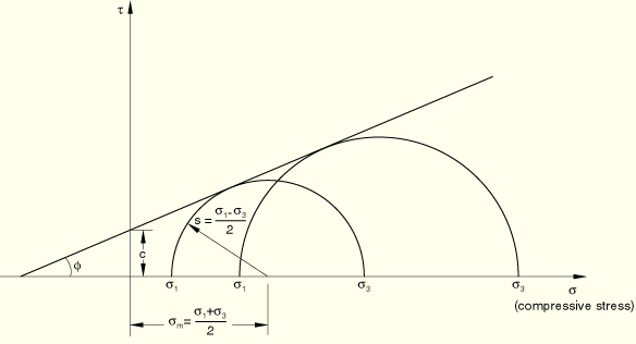
The Mohr-Coulomb criterion assumes that failure occurs when the shear stress on any point in a material reaches a value that depends linearly on the normal stress in the same plane. The Mohr-Coulomb model is based on plotting Mohr's circle for states of stress at failure in the plane of the maximum and minimum principal stresses. The failure line is the best straight line that touches these Mohr's circles (Figure 18.3.3–1).
Therefore, the Mohr-Coulomb model is defined by
![]()
![]()
Substituting for ![]() and
and ![]() , multiplying both sides by
, multiplying both sides by ![]() , and reducing, the Mohr-Coulomb model can be written as
, and reducing, the Mohr-Coulomb model can be written as
![]()
![]()
![]()
For general states of stress the model is more conveniently written in terms of three stress invariants as
![]()
![]()
![]()
is the slope of the Mohr-Coulomb yield surface in the p–![]() stress plane (see Figure 18.3.3–2), which is commonly referred to as the friction angle of the material and can depend on temperature and predefined field variables;
stress plane (see Figure 18.3.3–2), which is commonly referred to as the friction angle of the material and can depend on temperature and predefined field variables;
c
is the cohesion of the material; and
![]()
is the deviatoric polar angle defined as
![]()
![]()
is the equivalent pressure stress,
![]()
is the Mises equivalent stress,
![]()
is the third invariant of deviatoric stress,
![]()
is the deviatoric stress.
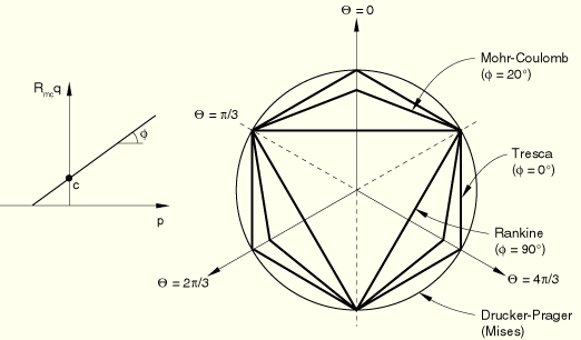
The friction angle ![]() controls the shape of the yield surface in the deviatoric plane as shown in Figure 18.3.3–2. The friction angle can range from
controls the shape of the yield surface in the deviatoric plane as shown in Figure 18.3.3–2. The friction angle can range from ![]() . In the case of
. In the case of ![]() the Mohr-Coulomb model reduces to the pressure-independent Tresca model with a perfectly hexagonal deviatoric section. In the case of
the Mohr-Coulomb model reduces to the pressure-independent Tresca model with a perfectly hexagonal deviatoric section. In the case of ![]() the Mohr-Coulomb model reduces to the “tension cut-off” Rankine model with a triangular deviatoric section and
the Mohr-Coulomb model reduces to the “tension cut-off” Rankine model with a triangular deviatoric section and ![]() (this limiting case is not permitted within the Mohr-Coulomb model described here).
(this limiting case is not permitted within the Mohr-Coulomb model described here).
While using one-element tests to verify the calibration of the model, it should be noted that the ABAQUS/Standard output variables SP1, SP2, and SP3 correspond to the principal stresses ![]() ,
, ![]() , and
, and ![]() , respectively.
, respectively.
The flow potential G is chosen as a hyperbolic function in the meridional stress plane and the smooth elliptic function proposed by Menétrey and Willam (1995) in the deviatoric stress plane:
![]()
![]()
![]()
![]()
is the dilation angle measured in the p–![]() plane at high confining pressure and can depend on temperature and predefined field variables;
plane at high confining pressure and can depend on temperature and predefined field variables;
![]()
is the initial cohesion yield stress, ![]() ;
;
![]()
is the deviatoric polar angle defined previously;
![]()
is a parameter, referred to as the meridional eccentricity, that defines the rate at which the hyperbolic function approaches the asymptote (the flow potential tends to a straight line in the meridional stress plane as the meridional eccentricity tends to zero); and
e
is a parameter, referred to as the deviatoric eccentricity, that describes the “out-of-roundedness” of the deviatoric section in terms of the ratio between the shear stress along the extension meridian (![]() ) and the shear stress along the compression meridian (
) and the shear stress along the compression meridian (![]() ).
).
By default, the deviatoric eccentricity, e, is calculated as
![]()
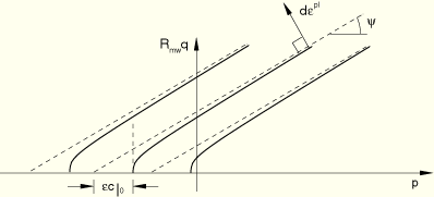
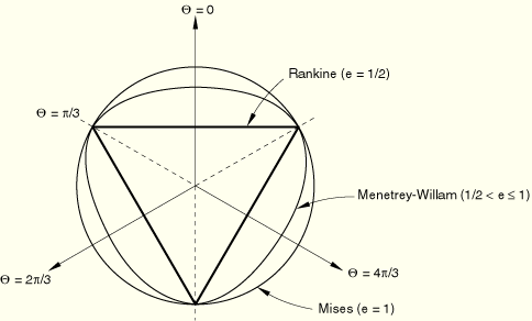
This flow potential, which is continuous and smooth, ensures that the flow direction is always uniquely defined. A family of hyperbolic potentials in the meridional stress plane is shown in Figure 18.3.3–3, and the flow potential in the deviatoric stress plane is shown in Figure 18.3.3–4.
Flow in the meridional stress plane can be close to associated when the angle of friction, ![]() , and the angle of dilation,
, and the angle of dilation, ![]() , are equal and the meridional eccentricity,
, are equal and the meridional eccentricity, ![]() , is very small; however, flow in this plane is, in general, nonassociated. Flow in the deviatoric stress plane is always nonassociated.
, is very small; however, flow in this plane is, in general, nonassociated. Flow in the deviatoric stress plane is always nonassociated.
| Input File Usage: | Use the following option to allow ABAQUS/Standard to calculate the value of e (default): |
*MOHR COULOMB Use the following option to specify the value of e directly: *MOHR COULOMB, DEVIATORIC ECCENTRICITY=e |
| ABAQUS/CAE Usage: | Use the following option to allow ABAQUS/Standard to calculate the value of e (default): |
Property module: material editor: Mechanical Use the following option to specify the value of e directly: Property module: material editor: Mechanical |
Since the plastic flow is nonassociated in general, the use of this Mohr-Coulomb model generally requires the unsymmetric matrix storage and solution scheme (see “Procedures: overview,” Section 6.1.1).
The Mohr-Coulomb plasticity model can be used with any stress/displacement elements in ABAQUS/Standard other than one-dimensional elements (beam and truss elements) or elements for which the assumed stress state is plane stress (plane stress, shell, and membrane elements).
In addition to the standard output identifiers available in ABAQUS/Standard (“ABAQUS/Standard output variable identifiers,” Section 4.2.1), the following variable has special meaning for the Mohr-Coulomb plasticity model:
PEEQ | Equivalent plastic strain, |