Product: ABAQUS/Explicit
Surface-based fluid-filled cavities are modeled by:
using standard finite elements to model the fluid-filled structure;
using a surface definition to provide the coupling between the deformation of the fluid-filled structure and the pressure exerted by the contained fluid on the cavity boundary of the structure;
defining the fluid behavior;
using fluid exchange definitions to model the transfer of fluid between a cavity and the environment or between multiple cavities; and
using inflator definitions to infuse a gas mixture into a fluid cavity to simulate the inflation of an automotive airbag.
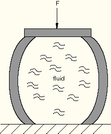
In certain applications it may be necessary to predict the mechanical response of a liquid-filled or a gas-filled structure. Examples include pressure vessels, hydraulic or pneumatic driving mechanisms, and automotive airbags. A primary difficulty in addressing such applications is the coupling between the deformation of the structure and the pressure exerted by the contained fluid on the structure. Figure 11.6.1–1 illustrates a simple example of a fluid-filled structure subjected to a system of external loads. The response of the structure depends not only on the external loads but also on the pressure exerted by the fluid, which, in turn, is affected by the deformation of the structure. The surface-based fluid cavity capability provides the coupling needed to analyze such situations. The cavity is assumed to be completely filled with fluid with the same properties and state; that is, effects such as sloshing and wave propagation through the fluid cannot be modeled with this feature.
The boundary of the fluid cavity is defined by an element-based surface with normals pointing to the inside of the cavity. The underlying elements can be standard solid or structural elements as well as surface elements. Surface elements can be used to model holes in the structure or to fill in rigid regions where rigid or other load-carrying elements do not exist (see “Surface elements,” Section 26.7.1). Care must be taken when using surface elements such that nodes completely surrounded by only surface elements have proper boundary conditions.
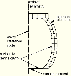
Consider the example presented in Figure 11.6.1–1. Solid elements are defined on the top and side of the cavity as indicated in Figure 11.6.1–2. A surface element is defined on the bottom rigid boundary of the cavity where no standard elements exist. The node located at the intersection of the axis of symmetry and the lower rigid boundary of the cavity must be restrained in the r- and z-directions because it is connected only to a surface element. The surface defining the cavity is based on the underlying solid and surface elements.
An additional volume can be added to the actual volume of the cavity calculated by ABAQUS/Explicit. If the boundary of the cavity is not defined by an element-based surface, the fluid cavity is assumed to have a fixed volume that is equal to the added volume.
A single node, known as the cavity reference node, is associated with a fluid cavity. This cavity reference node has a single degree of freedom representing the pressure inside the fluid cavity. The cavity reference node is also used in calculating the cavity volume.
If the cavity is not bounded by symmetry planes, the surface defining the cavity must completely enclose the cavity to ensure proper calculation of its volume. In this case the location of the cavity reference node is arbitrary and does not have to lie inside the cavity.
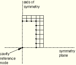
If, as a result of symmetry, only a portion of the cavity boundary is modeled with standard elements, the cavity reference node must be located on the symmetry plane or axis (Figure 11.6.1–2). If multiple symmetry planes exist, the cavity reference node must be located on the intersection of the symmetry planes (Figure 11.6.1–3). For an axisymmetric analysis the cavity reference node must be located on the axis of symmetry. These requirements are a consequence of the fluid cavity not being fully enclosed by the surface defining the cavity.
The behavior of the fluid within the fluid-filled cavity can be based either on a hydraulic or a pneumatic model. The hydraulic model can simulate nearly incompressible fluid behavior. The compressibility is controlled by a bulk modulus. The pneumatic model is based on an ideal gas. The gas can be defined by multiple species, and you can specify the temperature of the gas or have ABAQUS/Explicit calculate it based on the assumption of adiabatic behavior. A multi-species ideal gas with an adiabatic temperature update is an appropriate model for automotive airbags.
There are many ways in ABAQUS/Explicit to model the transfer of fluid into or out of a cavity. The flow can be specified as a prescribed mass or volume flux history or can model physical mechanisms due to a pressure differential such as venting through an exhaust orifice or leakage through a porous fabric. Fluid exchange definitions are used for this purpose and can model flow between a fluid cavity and its environment or between two fluid cavities (see “Defining fluid exchange,” Section 11.6.3, for details). ABAQUS also has the capability to model inflators used for the deployment of automotive airbags. Conditions at the inflator can be specified directly or tank test data can be used (see “Defining inflators,” Section 11.6.4, for details).
Many fluid-filled systems such as airbags have multiple chambers with fluid flowing between chambers through holes or fabric leakage. In other cases it is advantageous to divide a single physical chamber into multiple chambers with fictitious walls to model a gradient in pressure across the physical chamber. Some fictitious leakage mechanisms through inter-chamber walls can be defined to obtain reasonable behavior. This can be a useful modeling technique when simulating the complex unfolding of an airbag. To model multiple chambers, define a fluid cavity for each chamber and link the fluid cavities together with the appropriate fluid exchange definitions. Averaged properties for the multi-chambered model can be output if requested (see “Defining fluid cavities,” Section 11.6.2, for details).
The inertia of the fluid inside a fluid cavity or fluid exchanged between cavities is not automatically taken into account. To add the effect of inertia, use MASS elements on the boundary of the cavity. You should make sure that the total added mass corresponds to the mass of the fluid in the cavity and that the distribution of the MASS elements is a reasonable representation of the distributed fluid mass for the type of loading to which the structure is subjected. Only the overall effect of the fluid inertia can be modeled; the constant pressure assumption in the cavity makes it impossible to model any pressure gradient-driven fluid motions. Thus, the approach assumes that the time scale of the excitation is very long compared to typical response times for the fluid.
If a large amount of fluid is removed from a cavity or the material surrounding the cavity is very flexible, the cavity may partially collapse and portions of the cavity walls may contact each other. Self-contact of the cavity walls and contact with surrounding structures can be handled effectively by using the general contact algorithm (see “Defining general contact interactions,” Section 29.3.1). ABAQUS/Explicit can also account for the blockage of flow out of a cavity due to contacting surfaces (see “Accounting for blockage due to contacting boundary surfaces” in “Defining fluid exchange,” Section 11.6.3).
The initial fluid pressure and temperature can be specified (see “Initial conditions,” Section 27.2.1). For an ideal gas the initial pressure represents the gauge pressure over and above the ambient pressure. The initial temperature should be given in the temperature scale used. Absolute zero in that temperature scale is specified separately for an ideal gas (see “Defining fluid cavities,” Section 11.6.2).
If membrane elements are used as the underlying elements for the fluid cavity, the reference mesh (initial metric) can also be specified (see “Initial conditions,” Section 27.2.1).
The pressure degree of freedom at the cavity reference node (degree of freedom number 8) is a primary variable in the problem. Thus, it can be prescribed by defining a boundary condition (see “Boundary conditions,” Section 27.3.1), similar to the way displacements can be prescribed. Prescribing the pressure at the cavity reference node is equivalent to applying a uniform pressure to the cavity boundary using a distributed load definition (see “Distributed loads,” Section 27.4.3).
If the pressure is prescribed with a boundary condition, the fluid volume is adjusted automatically to fill the cavity (that is, fluid is assumed to enter and leave the cavity as needed to maintain the prescribed pressure). This behavior is useful in situations where a cavity is deformed prior to the introduction of the effect of the fluid. In a subsequent step you can remove the boundary condition on the pressure degree of freedom (see “Removing boundary conditions” in “Boundary conditions,” Section 27.3.1), thus “sealing” the cavity with the current fluid volume.
Distributed pressures and body forces, as well as concentrated nodal forces, can be applied to the fluid-filled structure, as described in “Concentrated loads,” Section 27.4.2, and “Distributed loads,” Section 27.4.3.
Predefined temperature fields and user-defined field variables can be defined for both fluid-filled structures and the enclosed fluids, as described in “Predefined fields,” Section 27.6.1.
Fluid temperatures can be specified at all cavity reference nodes as predefined fields (see “Predefined temperature” in “Predefined fields,” Section 27.6.1), unless an adiabatic process is specified or a coupled temperature-displacement procedure is used. Any difference between the applied and initial temperatures will cause thermal expansion for a pneumatic fluid and for a hydraulic fluid if a thermal expansion coefficient is given. A specified temperature field can also affect temperature-dependent material properties, if any exist, for both fluid-filled structures and enclosed fluids.
The values of user-defined field variables can be specified at all cavity reference nodes (see “Predefined field variables” in “Predefined fields,” Section 27.6.1). These values will affect field-variable-dependent material properties for the enclosed fluid.
The state of the fluid inside the cavity is available for history output using the nodal output variables PCAV, CVOL, CTEMP, CSAREA, and CMASS, which represent the gauge fluid pressure, cavity volume, cavity temperature, cavity surface area, and mass of the fluid, respectively. Output variable CTEMP is available only when an ideal gas model is used under adiabatic conditions. If the node set for which the output request is made contains more than one fluid cavity, the time histories of the average fluid pressure, total volume, average fluid temperature, sum of all the external cavity surface areas, and total mass of these cavities will also be output by using the nodal output variables APCAV, TCVOL, ACTEMP, TCSAREA, and TCMASS, respectively.
When the model includes fluid exchange definitions, use nodal output variables CMFL and CMFLT to obtain history output of the total mass flow rate and total accumulated mass flow out of a cavity and CEFL and CEFLT to obtain history output of the total heat energy flow rate and total accumulated heat energy flow out of a cavity. If more than one fluid exchange is defined for a cavity, time histories of the mass or heat energy flow rate and accumulated mass or heat energy flow out of the cavity for each fluid exchange will also be output.
If the fluid cavity is modeled by a mixture of ideal gases, time histories of the molecular mass fraction of each fluid species inside the fluid cavity can be obtained by using nodal output variable CMF.
If inflators are used, use nodal output variables MINFL, MINFLT, and TINFL to obtain time histories of mass flow rate, accumulated mass flow, and inflator temperature for each inflator definition (see “ABAQUS/Explicit output variable identifiers,” Section 4.2.2).
*HEADING
…
*FLUID CAVITY, NAME=cavity_name, BEHAVIOR=behavior_name,
REF NODE=cavity_reference_node, SURFACE=surface_name
*FLUID BEHAVIOR, NAME=behavior_name
*FLUID DENSITY
Data line to define density
*FLUID BULK MODULUS
Data line to define  bulk modulus
*FLUID EXPANSION
Data line to define thermal expansion
**
*FLUID EXCHANGE, NAME=exchange_name, PROPERTY=exchange_property_name
cavity_reference_node
*FLUID EXCHANGE PROPERTY, NAME=exchange_property_name, TYPE=MASS FLUX
Data line to define mass flow rate per unit area
**
*INITIAL CONDITIONS, TYPE=TEMPERATURE
Data line to define initial temperature
*INITIAL CONDITIONS, TYPE=FLUID PRESSURE
Data line to define initial pressure
**
*STEP
**
*TEMPERATURE
Data line to define temperature
*FLUID EXCHANGE ACTIVATION
exchange_name
**
*END STEP
*HEADING
…
*FLUID CAVITY, NAME=chamber_1, MIXTURE=MOLAR FRACTION, ADIABATIC,
REF NODE=chamber_1_reference_node, SURFACE=surface_name_1
blank line
Oxygen,  0.2
Nitrogen,  0.75
Carbon_dioxide,  0.05
**
*FLUID CAVITY, NAME=chamber_2, BEHAVIOR=Air, ADIABATIC,
REF NODE=chamber_2_reference_node, SURFACE=surface_name_2
blank line
**
*FLUID BEHAVIOR, NAME=Air
*CAPACITY, TYPE=POLYNOMIAL
Data line to define heat capacity coefficient
*MOLECULAR WEIGHT
Data line to define molecular weight
**
*FLUID BEHAVIOR, NAME=Oxygen
*CAPACITY, TYPE=POLYNOMIAL
Data line to define heat capacity coefficient
*MOLECULAR WEIGHT
Data line to define molecular weight
**
*FLUID BEHAVIOR, NAME=Nitrogen
*CAPACITY, TYPE=POLYNOMIAL
Data line to define heat capacity coefficient
*MOLECULAR WEIGHT
Data line to define molecular weight
**
*FLUID BEHAVIOR, NAME=Carbon_dioxide
*CAPACITY, TYPE=POLYNOMIAL
Data line to define heat capacity coefficient
*MOLECULAR WEIGHT
Data line to define molecular weight
**
*FLUID INFLATOR, NAME=inflator, PROPERTY=inflator_property
chamber_1_reference_node
*FLUID INFLATOR PROPERTY, NAME=inflator_property,
TYPE=MASS TEMPERATURE
Data lines to define mass flow rate and gas temperature
*FLUID INFLATOR MIXTURE, TYPE=MOLAR FRACTION, NUMBER SPECIES=2
Carbon_dioxide, Nitrogen
Table to define molecular mass fraction
**
*FLUID EXCHANGE, NAME=exhaust, PROPERTY=exhaust_behavior
chamber_1_reference_node
*FLUID EXCHANGE PROPERTY, NAME=exhaust_behavior, TYPE=ORIFICE
Data line to specify orifice behavior
*FLUID EXCHANGE, NAME=leakage_1, PROPERTY=fabric_behavior
chamber_1_reference_node
*FLUID EXCHANGE, NAME=leakage_2, PROPERTY=fabric_behavior
chamber_2_reference_node
*FLUID EXCHANGE PROPERTY, NAME=fabric_behavior, TYPE=FABRIC LEAKAGE
Data line to specify fabric leakage behavior
**
*FLUID EXCHANGE, NAME=chamber_wall, PROPERTY=wall_behavior,
EFFECTIVE AREA=
chamber_1_reference_node, chamber_2_reference_node
*FLUID EXCHANGE PROPERTY, NAME=wall_behavior, TYPE=ORIFICE
Data line to specify orifice behavior
**
*AMPLITUDE, NAME=amplitude_name
Data line to define amplitude variations
*PHYSICAL CONSTANTS, UNIVERSAL GAS CONSTANT=
**
*INITIAL CONDITIONS, TYPE=FLUID PRESSURE
Data line to define initial pressure
*INITIAL CONDITIONS, TYPE=TEMPERATURE
Data line to define initial temperature
**
*STEP
**
*FLUID EXCHANGE ACTIVATION
exhaust, leakage_1, leakage_2,  chamber_wall
*FLUID INFLATOR ACTIVATION, INFLATION TIME AMPLITUDE=amplitude_name
inflator
**
*END STEP