Products: ABAQUS/Standard ABAQUS/Explicit
Fluid-filled cavities are modeled by:
using standard finite elements to model the fluid-filled structure;
using hydrostatic fluid elements to provide the coupling between the deformation of the fluid-filled structure and the pressure exerted by the contained fluid on the cavity boundary of the structure;
defining the hydrostatic fluid properties; and
using fluid link elements to model the transfer of fluid between multiple fluid cavities or between a cavity and the environment, if necessary.
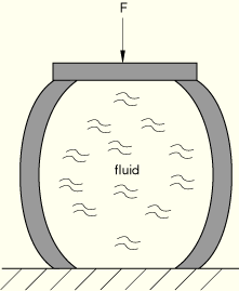
In certain applications it may be necessary to predict the mechanical response of a fluid-filled or a gas-filled structure. A primary difficulty in addressing such applications is the coupling between the deformation of the structure and the pressure exerted by the contained fluid or gas on the structure. Figure 11.5.1–1 illustrates a simple example of a fluid-filled structure subjected to a system of external loads. The response of the structure depends not only on the external loads but also on the pressure exerted by the fluid, which, in turn, is affected by the deformation of the structure. The hydrostatic fluid elements provide the coupling needed to analyze such situations. The cavity is assumed to be completely filled with fluid; that is, effects such as sloshing cannot be modeled.
Hydrostatic fluid elements are surface elements that cover the boundary of the fluid cavity. In regions where standard finite elements are used to model the boundary of the cavity, the hydrostatic fluid elements share the nodes at the cavity boundary with the standard elements.
Consider the example presented in Figure 11.5.1–1.
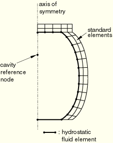
Hydrostatic fluid elements are defined around the cavity boundary as indicated in Figure 11.5.1–2. A hydrostatic fluid element is also defined along the bottom rigid boundary of the cavity, even though no standard elements exist along this boundary. This fluid element is needed to define the cavity completely and to ensure proper calculation of its volume.All hydrostatic fluid elements associated with a given cavity share a common node known as the cavity reference node. This cavity reference node has a single degree of freedom representing the pressure inside the fluid cavity. The cavity reference node is also used in calculating the cavity volume.
If the cavity is not bounded by symmetry planes, it must be completely enclosed with hydrostatic fluid elements. In this case the location of the cavity reference node is arbitrary and does not have to lie inside the cavity.
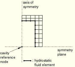
If as a result of symmetry only a portion of the cavity boundary is modeled with standard elements, the cavity reference node must be located on the symmetry plane or axis (Figure 11.5.1–2). If multiple symmetry planes exist, the cavity reference node must be located on the intersection of the symmetry planes (Figure 11.5.1–3). For an axisymmetric analysis the cavity reference node must be located on the axis of symmetry. These requirements are a consequence of the fluid cavity not being fully enclosed with hydrostatic fluid elements.
If hydrostatic fluid elements are defined with nodes that are not attached to standard elements, proper displacement boundary conditions must be applied to these nodes. Thus, in the example shown in Figure 11.5.1–2, the node located at the intersection of the axis of symmetry and the lower rigid boundary of the cavity must be restrained in the r- and z-directions.
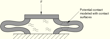
If a large amount of fluid is removed from a cavity or the material surrounding the cavity is very flexible, the cavity may partially collapse and portions of the cavity walls may contact each other (see Figure 11.5.1–4). Interior contact can be simulated by defining contact surfaces on the sections of the cavity wall where contact occurs. In ABAQUS/Standard master-slave and self-contact can be modeled (see “Defining contact pairs in ABAQUS/Standard,” Section 29.2.1). In ABAQUS/Explicit either single- or multiple-surface contact can be used to avoid unrealistic overclosure of the cavity.
It is possible that a particular application may involve multiple fluid cavities with potential transfer of fluid between the cavities due to a pressure differential. This situation can be analyzed by defining one or more fluid link elements between the cavity reference nodes. The mass flow rate through the link can be defined as a function of pressure differential, average pressure, average temperature, and external field variables. Fluid transfer between a cavity and the environment can be modeled if one side of the link is unconnected and the pressure at that end is prescribed with a boundary condition.
While the hydrostatic fluid elements and fluid link elements can be used in a dynamic procedure, the inertia of the fluid is not taken into account. To add the effect of inertia, use MASS elements on the boundary of the cavity. You should make sure that the total added mass corresponds to the mass of the fluid in the cavity and that the distribution of the masses is a reasonable representation of the distributed fluid mass for the type of loading to which the structure is subjected. Only the overall effect of the fluid inertia can be modeled; the constant pressure assumption in the cavity makes it impossible to model any pressure gradient-driven fluid motions. Thus, the approach assumes that the time scale of the excitation is very long compared to typical response times for the fluid.
In some hydrostatic fluid element applications in ABAQUS/Standard, negative eigenvalues may be encountered during the solution. These negative eigenvalues do not necessarily indicate that a bifurcation or buckling load has been exceeded. If the predicted response otherwise appears to be reasonable, these messages can be ignored. A detailed description of how negative eigenvalues can develop during the solution of hydrostatic fluid element problems is presented in “Hydrostatic fluid elements,” Section 3.8.1 of the ABAQUS Theory Manual.
Hydrostatic fluid elements can be used in all procedures except coupled pore fluid diffusion/stress analysis (see “Coupled pore fluid diffusion and stress analysis,” Section 6.7.1).
The initial fluid pressure and, in ABAQUS/Standard, initial temperature can be specified (see “Initial conditions,” Section 27.2.1).
The pressure degree of freedom at the cavity reference node (degree of freedom number 8) is a primary variable in the problem. Thus, it can be prescribed by defining a boundary condition (see “Boundary conditions,” Section 27.3.1), similar to the way displacements can be prescribed. Prescribing the pressure at the cavity reference node is equivalent to applying a uniform pressure to the cavity boundary using a distributed load definition (see “Distributed loads,” Section 27.4.3).
If the pressure is prescribed with a boundary condition, the fluid volume is automatically adjusted to fill the cavity (that is, fluid is assumed to enter and leave the cavity as needed to maintain the prescribed pressure). This behavior is useful in situations where a cavity is deformed prior to the introduction of a fluid. In a subsequent step you can remove the boundary condition on the pressure degree of freedom (see “Removing boundary conditions” in “Boundary conditions,” Section 27.3.1), thus “sealing” the cavity with the current fluid volume.
Distributed pressures and body forces, as well as concentrated nodal forces, can be applied to the fluid-filled structure, as described in “Concentrated loads,” Section 27.4.2, and “Distributed loads,” Section 27.4.3.
A prescribed quantity of fluid can be added to or removed from a cavity during the analysis by specifying a mass flow rate, q. A positive value for q adds fluid to the cavity, while a negative value removes fluid from the cavity.
The mass flow rate for a fluid cavity cannot be specified in random response or steady-state dynamic procedures.
The amount of fluid in the cavity will also change if the cavity pressure is prescribed with a boundary condition as described above. If the boundary condition is subsequently removed, the amount of fluid in the cavity will change only if fluid link elements are connected to, or a mass flow rate is defined for, the cavity reference node.
| Input File Usage: | *FLUID FLUX cavity reference node number or node set name, q |
By default, the mass flow rate will be applied instantaneously at the beginning of the step and left unchanged for the duration of the step, regardless of the procedure being used in the step. Alternatively, you can specify the variation of the rate throughout the step by referring to an amplitude curve (see “Amplitude curves,” Section 27.1.2).
| Input File Usage: | *FLUID FLUX, AMPLITUDE=name |
Predefined temperature fields and user-defined field variables can be defined for both fluid-filled structures and the enclosed fluids, as described in “Predefined fields,” Section 27.6.1.
Nodal temperatures can be specified as predefined fields (see “Predefined temperature” in “Predefined fields,” Section 27.6.1). When specifying the temperature of an enclosed fluid, the cavity reference node must be used to define the uniform temperature of the fluid.
In ABAQUS/Standard an initial temperature can be specified for a fluid-filled structure. Any difference between the applied and initial temperatures will cause thermal strain if a thermal expansion coefficient is given for the material (“Thermal expansion,” Section 20.1.2). If a thermal expansion coefficient is given for an enclosed fluid, such a difference in temperatures will result in a change in fluid volume and fluid density, as discussed in “Hydrostatic fluid models,” Section 20.4.1.
A defined temperature field can also affect temperature-dependent material properties, if any exist, for both fluid-filled structures and enclosed fluids.
The values of user-defined field variables can be specified (see “Predefined field variables” in “Predefined fields,” Section 27.6.1). These values will affect field-variable-dependent material properties for both the fluid-filled structure and the enclosed fluid, if any exist.
The fluid within a fluid-filled cavity must be modeled by using one of the hydrostatic fluid models (“Hydrostatic fluid models,” Section 20.4.1). The following properties can be defined for a fluid: bulk modulus; density; and, in ABAQUS/Standard, coefficient of thermal expansion. The structure itself can be modeled using any elastic or inelastic material model.
Fluid-filled cavities are modeled using hydrostatic fluid elements (“Hydrostatic fluid elements,” Section 26.8.1) and, if necessary, fluid link elements (“Fluid link elements,” Section 26.8.3).
The fluid pressure and cavity volume can be obtained at the reference node of the hydrostatic fluid elements (output variables PCAV and CVOL, respectively). For results and data file output in steady-state dynamic procedures the magnitude and phase angle of the fluid pressure can be obtained as nodal variable PPOR.
In ABAQUS/Standard, if fluid flows between cavities or between a cavity and the environment, the mass flow rate and total mass flow can be obtained (output variables MFL and MFLT, respectively). For results and data file output in direct-solution steady-state dynamic procedures the magnitude and phase angle of the mass flow rate and total mass flow can be obtained (output variables PHMFL and PHMFT, respectively).
The following is an example of a hydrostatic fluid analysis:
*HEADING
…
*ELEMENT, TYPE=hydrostatic fluid element, ELSET=name_1
…
*ELEMENT, TYPE=fluid link element, ELSET=name_2
…
Define the hydrostatic fluid behavior
*PHYSICAL CONSTANTS, ABSOLUTE ZERO=
*FLUID PROPERTY, ELSET=name_1, REF NODE=number, TYPE=fluid type
The TYPE parameter is applicable only in an ABAQUS/Standard analysis.
…
*FLUID DENSITY
…
Define the compressibility and thermal expansion coefficient for a hydraulic fluid (available only
in ABAQUS/Standard)
*FLUID BULK MODULUS
…
*FLUID EXPANSION
…
Define the fluid link properties
*FLUID LINK, ELSET=name_2
…
Specify the initial conditions
*INITIAL CONDITIONS, TYPE=TEMPERATURE
…
*INITIAL CONDITIONS, TYPE=FLUID PRESSURE
…
**
*STEP
…
Change the temperature of the fluid
*TEMPERATURE
…
Change the amount of fluid in a cavity
*FLUID FLUX
…
*END STEP