Products: ABAQUS/Standard ABAQUS/CAE
ABAQUS/Standard offers the evaluation of several parameters for fracture mechanics studies:
the J-integral, which is widely accepted as a quasi-static fracture mechanics parameter for linear material response and, with limitations, for nonlinear material response;
the ![]() -integral, which has an equivalent role to the J-integral in the context of time-dependent creep behavior (“Rate-dependent plasticity: creep and swelling,” Section 18.2.4) in a quasi-static step (“Quasi-static analysis,” Section 6.2.5);
-integral, which has an equivalent role to the J-integral in the context of time-dependent creep behavior (“Rate-dependent plasticity: creep and swelling,” Section 18.2.4) in a quasi-static step (“Quasi-static analysis,” Section 6.2.5);
the stress intensity factors, which are used in linear elastic fracture mechanics to measure the strength of the local crack-tip fields;
the crack propagation direction—i.e., the angle at which a preexisting crack will propagate; and
the T-stress, which represents a stress parallel to the crack faces and is used as an indicator of the extent to which parameters like the J-integral are useful characterizations of the deformation field around the crack.
are output quantities—they do not affect the results;
are valid in two and three dimensions;
can be used only with quadrilateral elements (in two dimensions) or brick elements (in three dimensions); and
can be requested only in general analysis steps.
Several contour integral evaluations are possible at each location along a crack. In a finite element model each evaluation can be thought of as the virtual motion of a block of material surrounding the crack tip (in two dimensions) or surrounding each node along the crack line (in three dimensions). Each such block is defined by contours: each contour is a ring of elements completely surrounding the crack tip or the nodes along the crack line from one crack face to the opposite crack face. These rings of elements are defined recursively to surround all previous contours.
ABAQUS/Standard automatically finds the elements that form each ring from the regions given as the crack-tip or crack-line definition. Each contour provides an evaluation of the contour integral. The number of evaluations possible is the number of such rings of elements. You must specify the number of contours to be used in calculating contour integrals. In addition, you select the type of contour integral to be calculated, as described below. The default is to calculate the J-integral.
You can assign a name to a crack for its contour integral calculation. This name can be used to identify the contour integral values in the data file and the output database file. It is also used in ABAQUS/CAE to request contour integral output.
If you do not specify a crack name, by default ABAQUS/Standard will generate crack numbers automatically following the order in which the cracks are defined.
| Input File Usage: | *CONTOUR INTEGRAL, CRACK NAME=crack name, CONTOURS=n, TYPE=integral_type |
| ABAQUS/CAE Usage: | Interaction module: Special |
Using the divergence theorem, the contour integral can be expanded into an area integral in two dimensions or a volume integral in three dimensions, over a finite domain surrounding the crack. This domain integral method is used to evaluate contour integrals in ABAQUS/Standard. The method is quite robust in the sense that accurate contour integral estimates are usually obtained even with quite coarse meshes; because the integral is taken over a domain of elements surrounding the crack, errors in local solution parameters have less effect on the evaluated quantities such as J, ![]() , the stress intensity factors, and the T-stress.
, the stress intensity factors, and the T-stress.
Contour integrals at several different crack tips in two dimensions or along several different crack lines in three dimensions can be evaluated at any time by repeating the contour integral request as often as needed in the step definition. You must specify the crack front and the direction of virtual crack extension (or the normal to the crack plane if this normal is constant) for each crack tip or crack line, as described below. In addition, you must specify the number of contours to be calculated for each integral.
The J-integral is usually used in rate-independent quasi-static fracture analysis to characterize the energy release associated with crack growth. It can be related to the stress intensity factor if the material response is linear.
The J-integral is defined in terms of the energy release rate associated with crack advance. For a virtual crack advance ![]() in the plane of a three-dimensional fracture, the energy release rate is given by
in the plane of a three-dimensional fracture, the energy release rate is given by
![]()
![]()
Initial stresses are not considered in the definition of contour integrals. Therefore, contour integral calculations for analyses including initial stresses in the regions used for the contour integral calculations will not be correct.
| Input File Usage: | *CONTOUR INTEGRAL, CONTOURS=n, TYPE=J |
| ABAQUS/CAE Usage: | Step module: history output request editor: Domain: Contour integral name: crack name, Number of contours: n, Type: J-integral |
The J-integral should be independent of the domain used provided that the crack faces are parallel to each other, but J-integral estimates from different rings may vary because of the approximate nature of the finite element solution. Strong variation in these estimates, commonly called domain dependence or contour dependence, typically indicates an error in the contour integral definition. Gradual variation in these estimates may indicate that a finer mesh is needed or, if plasticity is included, that the contour integral domain does not completely include the plastic zone. If the “equivalent elastic material” is not a good representation of the elastic-plastic material, the contour integrals will be domain independent only if they completely include the plastic zone. Since it is not always possible to include the plastic zone in three dimensions, a finer mesh may be the only solution.
If the first contour integral is defined by specifying the nodes at the crack tip, the first few contours may be inaccurate. To check the accuracy of these contours, you can request more contours and determine the value of the contour integral that appears approximately constant from one contour to the next. The contour integral values that are not approximately equal to this constant should be discarded. In linear elastic problems the first and second contours typically should be ignored as inaccurate.
The ![]() -integral can be used for time-dependent creep behavior, where it characterizes creep crack deformation under certain creep conditions, including transient crack growth.
-integral can be used for time-dependent creep behavior, where it characterizes creep crack deformation under certain creep conditions, including transient crack growth. ![]() is, for example, proportional to the rate of growth of the crack-tip/crack-line creep zone for a stationary crack under small-scale creep conditions. Under steady-state creep conditions, when creep dominates throughout the specimen,
is, for example, proportional to the rate of growth of the crack-tip/crack-line creep zone for a stationary crack under small-scale creep conditions. Under steady-state creep conditions, when creep dominates throughout the specimen, ![]() becomes path independent and is known as
becomes path independent and is known as ![]() .
. ![]() -integrals should be requested only in a quasi-static step.
-integrals should be requested only in a quasi-static step.
The ![]() -integral is obtained by replacing the displacements with velocities and the strain energy density with the strain energy rate density in the J-integral expansion. The strain energy rate density is defined as
-integral is obtained by replacing the displacements with velocities and the strain energy density with the strain energy rate density in the J-integral expansion. The strain energy rate density is defined as
![]()
![]()
For the hyperbolic-sine law an analytical expression of ![]() is not available. For this law
is not available. For this law ![]() is obtained by numerical integration; a five-point Gauss quadrature scheme gives reasonable accuracy in the range of realistic creep strain rates.
is obtained by numerical integration; a five-point Gauss quadrature scheme gives reasonable accuracy in the range of realistic creep strain rates.
The domain integral method is used for ![]() -integrals as described above for J-integrals.
-integrals as described above for J-integrals.
For user-defined creep laws the strain energy rate density must be defined in user subroutine CREEP.
| Input File Usage: | *CONTOUR INTEGRAL, CONTOURS=n, TYPE=C |
| ABAQUS/CAE Usage: | Step module: history output request editor: Domain: Contour integral name: crack name, Number of contours: n, Type: Ct-integral |
Prior to steady state ![]() -integral estimates will exhibit domain dependence, even if the finite element mesh is sufficiently refined, because of the assumption of creep dominance within the domain specified. These
-integral estimates will exhibit domain dependence, even if the finite element mesh is sufficiently refined, because of the assumption of creep dominance within the domain specified. These ![]() estimates should be extrapolated to zero radius to obtain an improved
estimates should be extrapolated to zero radius to obtain an improved ![]() estimate corresponding to a contour shrunk onto the crack tip or crack line (see “Ct-integral evaluation,” Section 1.15.6 of the ABAQUS Benchmarks Manual).
estimate corresponding to a contour shrunk onto the crack tip or crack line (see “Ct-integral evaluation,” Section 1.15.6 of the ABAQUS Benchmarks Manual).
The stress intensity factors ![]() ,
, ![]() , and
, and ![]() are usually used in linear elastic fracture mechanics to characterize the local crack-tip/crack-line stress and displacement fields. They are related to the energy release rate (the J-integral) through
are usually used in linear elastic fracture mechanics to characterize the local crack-tip/crack-line stress and displacement fields. They are related to the energy release rate (the J-integral) through
![]()
![]()
![]()
![]()
![]()
Although the energy release rate is calculated directly in ABAQUS/Standard, it is usually not straightforward to compute stress intensity factors from a known J-integral for mixed-mode problems. ABAQUS/Standard provides an interaction integral method to compute the stress intensity factors directly for a crack under mixed-mode loading. This capability is available for linear isotropic and anisotropic materials. The theory is described in detail in “Stress intensity factor extraction,” Section 2.16.2 of the ABAQUS Theory Manual.
In this case the J-integrals calculated from the stress intensity factors will also be output. These J-integral values may be slightly different from those estimated by requesting the J-integral directly, due to the different algorithms used for the calculations.
| Input File Usage: | *CONTOUR INTEGRAL, CONTOURS=n, TYPE=K FACTORS |
| ABAQUS/CAE Usage: | Step module: history output request editor: Domain: Contour integral name: crack name, Number of contours: n, Type: Stress intensity factors |
The stress intensity factors have the same domain dependence features as the J-integral.
For homogeneous, isotropic elastic materials the direction of cracking initiation can be calculated using one of the following three criteria: the maximum tangential stress criterion, the maximum energy release rate criterion, or the ![]() criterion.
criterion. ![]() is not taken into account in any of these criteria.
is not taken into account in any of these criteria.
Using either the condition ![]() or
or ![]() (where r and
(where r and ![]() are polar coordinates centered at the crack tip in a plane orthogonal to the crack line), we can obtain
are polar coordinates centered at the crack tip in a plane orthogonal to the crack line), we can obtain
The crack propagation angle ![]() will be output.
will be output.
| Input File Usage: | *CONTOUR INTEGRAL, CONTOURS=n, TYPE=K FACTORS, DIRECTION=MTS |
| ABAQUS/CAE Usage: | Step module: history output request editor: Domain: Contour integral name: crack name, Number of contours: n, Type: Stress intensity factors, Crack initiation criterion: Maximum tangential stress |
This criterion postulates that a crack initially propagates in the direction that maximizes the energy release rate.
The crack propagation angle ![]() will be output.
will be output.
| Input File Usage: | *CONTOUR INTEGRAL, CONTOURS=n, TYPE=K FACTORS, DIRECTION=MERR |
| ABAQUS/CAE Usage: | Step module: history output request editor: Domain: Contour integral name: crack name, Number of contours: n, Type: Stress intensity factors, Crack initiation criterion: Maximum energy release rate |
This criterion assumes that a crack initially propagates in the direction that makes ![]() .
.
The crack propagation angle ![]() will be output.
will be output.
| Input File Usage: | *CONTOUR INTEGRAL, CONTOURS=n, TYPE=K FACTORS, DIRECTION=KII0 |
| ABAQUS/CAE Usage: | Step module: history output request editor: Domain: Contour integral name: crack name, Number of contours: n, Type: Stress intensity factors, Crack initiation criterion: K11=0 |
The T-stress component represents a stress parallel to the crack faces at the crack tip. Its magnitude can alter not only the size and shape of the plastic zone but also the stress triaxiality ahead of the crack tip. It is, therefore, a useful indicator of whether measures of the strength of the crack-tip singularity (such as the J-integral or the stress intensity factors) are useful in characterizing a crack under a particular loading. In a linear elastic analysis the T-stress should be calculated using loads equal to the loads in the elastic-plastic analysis. See “T-stress extraction,” Section 2.16.3 of the ABAQUS Theory Manual, for more information.
| Input File Usage: | *CONTOUR INTEGRAL, CONTOURS=n, TYPE=T-STRESS |
| ABAQUS/CAE Usage: | Step module: history output request editor: Domain: Contour integral name: crack name, Number of contours: n, Type: T-stress |
In general, the T-stress has larger domain dependence or contour dependence than the J-integral and the stress intensity factors. Numerical tests suggest that the estimates from the first two rings of elements abutting the crack tip or crack line generally do not provide accurate results. Sufficient contours extending from the crack tip or crack line should be chosen so that the T-stress can be determined to be independent of the number of contours, within engineering accuracy.
To request contour integral output, you must define the crack front and specify the virtual crack extension direction.
You must specify the crack front; i.e., the region that defines the first contour. ABAQUS/Standard uses this region and one layer of elements surrounding it to compute the first contour integral. An additional layer of elements is used to compute each subsequent contour.
The crack front can be equivalent to the crack tip in two dimensions or the crack line in three dimensions; or it can be a larger region surrounding the crack tip or crack line, in which case it must include the crack tip or crack line.
If blunted crack tips are modeled, the crack front should include all the nodes going from one crack face to the other that would collapse onto the crack tip if the radius of the blunted tip were reduced to zero. Otherwise, the contour integral value will depend on the path until the contour region reaches the parallel crack faces.
| Input File Usage: | *CONTOUR INTEGRAL, CONTOURS=n Specify the crack front node set name on the data line; the format depends on the method you use to specify the virtual crack extension direction. |
For two-dimensional cases only one crack front node set (the crack front at the crack tip) must be specified. For three-dimensional cases you must repeat the data line to specify the crack front for each node (or cluster of focused nodes) along the crack line in order from one end of the crack to the other, including the midside nodes of second-order elements; it is not permissible to skip nodes along the crack line. |
| ABAQUS/CAE Usage: | Interaction module: Special |
By default, ABAQUS/Standard defines the crack tip as the first node specified for the crack front and the crack line as the sequence of first nodes specified for the crack front. The first node is the node with the smallest node number, unless the node set is generated as unsorted. Alternatively, you can specify the crack-tip node or crack-line nodes directly. This specification plays a critical role for a three-dimensional crack with a blunt crack tip.
ABAQUS/CAE cannot determine the crack tip or crack line automatically based on the specified crack front. However, if you select a point to define the crack front in two dimensions, the same point defines the crack tip; likewise, if you select edges to define the crack front in three dimensions, the same edges define the crack line. For all other cases you must define the crack tip or crack line directly.
| Input File Usage: | Use the following option to specify the crack-tip nodes directly: |
*CONTOUR INTEGRAL, CONTOURS=n, CRACK TIP NODES
Specify the crack front node set name and the crack tip node number or node set name on the data line; the format depends on the method you use to specify the virtual crack extension direction.
Repeat the data line for three-dimensional cases. |
| ABAQUS/CAE Usage: | Interaction module: Special |
Sometimes a crack line may form a closed loop (for example, when modeling a full penny-shaped crack without invoking symmetry conditions). In such cases the finite element mesh in the crack-tip region can be created with or without seams; i.e., linear constraint equations (“Linear constraint equations,” Section 28.2.1) or multi-point constraints (“General multi-point constraints,” Section 28.2.2) may or may not be used to tie two layers of nodes together.
If a crack line forms a closed loop, the starting node set of the crack front can be chosen arbitrarily and the other node sets defining the crack front must go around the crack front sequentially. The last node set defining the crack front must be the same as the first node set. If a closed loop is formed by creating coincident nodes that are then tied together by linear constraint equations and multi-point constraints, the node sets must be specified in order starting from one of the node sets involved in the constraint equation or multi-point constraint and terminating with the other node set.
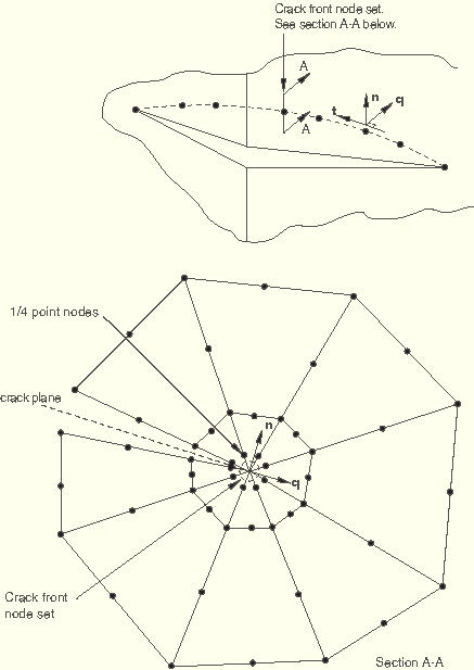
You must specify the direction of virtual crack extension at each crack tip in two dimensions or at each node along the crack line in three dimensions by specifying either the normal to the crack plane, ![]() , or the virtual crack extension direction,
, or the virtual crack extension direction, ![]() .
.
If the virtual crack extension direction is specified to point into the material (parallel to the crack faces), the contour integral values calculated will be positive. Negative contour values are obtained when the virtual crack extension direction is specified in the opposite direction.
The virtual crack extension direction can be defined by specifying the normal, ![]() , to the crack plane. In this case ABAQUS/Standard will calculate a virtual crack extension direction,
, to the crack plane. In this case ABAQUS/Standard will calculate a virtual crack extension direction, ![]() , that is orthogonal to the crack front tangent,
, that is orthogonal to the crack front tangent, ![]() , and the normal,
, and the normal, ![]() . As shown in Figure 11.4.2–1,
. As shown in Figure 11.4.2–1, ![]() for a three-dimensional crack; for a two-dimensional crack, we simply have
for a three-dimensional crack; for a two-dimensional crack, we simply have ![]() and
and ![]() . Specifying the normal implies that the crack plane is flat since only one value of
. Specifying the normal implies that the crack plane is flat since only one value of ![]() can be given per contour integral.
can be given per contour integral.
| Input File Usage: | *CONTOUR INTEGRAL, CONTOURS=n, NORMAL |
| ABAQUS/CAE Usage: | Interaction module: Special |
Alternatively, the virtual crack extension direction, ![]() , can be specified directly. In three dimensions the virtual crack extension direction,
, can be specified directly. In three dimensions the virtual crack extension direction, ![]() , will be corrected to be orthogonal to any normal defined at a node or in other cases to the tangent to the crack line itself. The tangent,
, will be corrected to be orthogonal to any normal defined at a node or in other cases to the tangent to the crack line itself. The tangent, ![]() , to the crack line at a particular point is obtained by parabolic interpolation through the crack front for which the virtual crack extension vector is defined and the nearest node sets on either side of this region. ABAQUS/Standard will normalize the virtual crack extension direction,
, to the crack line at a particular point is obtained by parabolic interpolation through the crack front for which the virtual crack extension vector is defined and the nearest node sets on either side of this region. ABAQUS/Standard will normalize the virtual crack extension direction, ![]() .
.
| Input File Usage: | *CONTOUR INTEGRAL, CONTOURS=n crack front node set name, |
Repeat the data line for three-dimensional cases to specify the crack front and virtual crack extension vector for each node (or cluster of focused nodes) along the crack line. |
| ABAQUS/CAE Usage: | Interaction module: Special |
In a case where the crack front intersects the external surface of a three-dimensional solid, where there is a surface of material discontinuity in the model, or where the crack is in a curved shell, the virtual crack extension direction, ![]() , must lie in the plane of the surface for accurate contour integral evaluation. Surface normals should be specified at all nodes that lie on such surfaces within the contours requested for this purpose (these nodes are printed out under the “Contour Integral” information in the data file). For shell element models the normals can be specified with the nodal coordinates if the normals calculated by ABAQUS/Standard are not adequate. For solid element models the normals can be specified either directly (see “Normal definitions at nodes,” Section 2.1.4, and “A plate with a part-through crack: elastic line spring modeling,” Section 1.4.1 of the ABAQUS Example Problems Manual) or using the nodal coordinates (the fourth–sixth coordinates). If surface normals are not specified for the nodes on the crack surfaces and the external surfaces at the ends of a crack line, ABAQUS/Standard will calculate the normals automatically for these nodes to correct any inadequate virtual crack extension directions,
, must lie in the plane of the surface for accurate contour integral evaluation. Surface normals should be specified at all nodes that lie on such surfaces within the contours requested for this purpose (these nodes are printed out under the “Contour Integral” information in the data file). For shell element models the normals can be specified with the nodal coordinates if the normals calculated by ABAQUS/Standard are not adequate. For solid element models the normals can be specified either directly (see “Normal definitions at nodes,” Section 2.1.4, and “A plate with a part-through crack: elastic line spring modeling,” Section 1.4.1 of the ABAQUS Example Problems Manual) or using the nodal coordinates (the fourth–sixth coordinates). If surface normals are not specified for the nodes on the crack surfaces and the external surfaces at the ends of a crack line, ABAQUS/Standard will calculate the normals automatically for these nodes to correct any inadequate virtual crack extension directions, ![]() .
.
If the crack is defined on a symmetry plane, only half the structure needs to be modeled. The change in potential energy calculated from the virtual crack front advance is doubled to compute the correct contour integral values.
| Input File Usage: | Use the following option to indicate that the crack is defined on a symmetry plane: |
*CONTOUR INTEGRAL, CONTOURS=n, SYMM |
| ABAQUS/CAE Usage: | Interaction module: Special |
Sharp cracks (where the crack faces lie on top of one another in the undeformed configuration) are usually modeled using small-strain assumptions. Focused meshes, as shown in Figure 11.4.2–1, should normally be used for small-strain fracture mechanics evaluations. However, for a sharp crack the strain field becomes singular at the crack tip. This result is obviously an approximation to the physics; however, the large-strain zone is very localized, and most fracture mechanics problems can be solved satisfactorily using only small-strain analysis.
The crack-tip strain singularity depends on the material model used. Linear elasticity, perfect plasticity, and power-law hardening are commonly used in fracture mechanics analysis. Power-law hardening has the form
![]()
Results for pure power-law nonlinear elastic materials in a body under traction loading are proportional to the load to some power. Therefore, the fracture parameters for one geometry under a particular load can be scaled to any other load of the same distribution but different magnitude.
If the loading is proportional (the direction of the stress increase in stress space is approximately constant) and monotonically increasing, power-law hardening deformation plasticity and incremental plasticity are essentially equivalent. However, deformation plasticity is a nonlinear elastic material for which more analytical results are available. ABAQUS uses the Ramberg-Osgood form of deformation plasticity (see “Deformation plasticity,” Section 18.2.13); this model is not a pure power law model, which must be considered.
In most cases the singularity at the crack tip should be considered in small-strain analysis (when geometric nonlinearities are ignored). Including the singularity often improves the accuracy of the J-integral, the stress intensity factors, and the stress and strain calculations because the stresses and strains in the region close to the crack tip are more accurate. If r is the distance from the crack tip, the strain singularity in small-strain analysis is
The square root and ![]() singularity can be built into a finite element mesh using standard elements. The crack tip is modeled with a ring of collapsed quadrilateral elements, as shown in Figure 11.4.2–2.
singularity can be built into a finite element mesh using standard elements. The crack tip is modeled with a ring of collapsed quadrilateral elements, as shown in Figure 11.4.2–2.
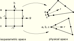
To obtain a mesh singularity, generally second-order elements are used and the elements are collapsed as follows:
Collapse one side of an 8-node isoparametric element (CPE8R, for example) so that all three nodes—a, b, and c—have the same geometric location (on the crack tip).
Move the midside nodes on the sides connected to the crack tip to the 1/4 point nearest the crack tip. You can create “quarter point” spacing with second-order isoparametric elements when you generate nodes for a region of a mesh; see “Creating quarter-point spacing” in “Node definition,” Section 2.1.1.
![]()
If 4-node isoparametric elements (for example, CPE4R) are used, one side of the element is collapsed, and the two coincident nodes are free to displace independently, a ![]() singularity is created.
singularity is created.
If the crack region is meshed with linear elements, the position specified for the midside nodes is ignored.
If nodes a, b, and c are constrained to move together, ![]() and the strains and stresses are square root singular (suitable for linear elasticity).
and the strains and stresses are square root singular (suitable for linear elasticity).
| Input File Usage: | *NFILL, SINGULAR |
Constrain the collapsed nodes to move together by specifying the same node number in the list of nodes forming the element or by using a linear constraint equation or multi-point constraint to tie them together. |
| ABAQUS/CAE Usage: | Interaction module: Special |
If the midside nodes remain at the midside points rather than being moved to the 1/4 points and nodes a, b, and c are allowed to move independently, only the ![]() singularity in strain is created (suitable for perfect plasticity).
singularity in strain is created (suitable for perfect plasticity).
| Input File Usage: | *NFILL |
| ABAQUS/CAE Usage: | Interaction module: Special |
If the midside nodes are moved to the 1/4 points but nodes a, b, and c are allowed to move independently, the singularity created is a combination of the square root and ![]() singularities. This combination is usually best for a power-law hardening material. However, since the
singularities. This combination is usually best for a power-law hardening material. However, since the ![]() singularity dominates, moving the midside nodes to the 1/4 points gives only slightly better results than if the nodes are left at the midside points. Since creating a mesh with the midside nodes moved to the quarter points can be difficult, it is often best to simply use the
singularity dominates, moving the midside nodes to the 1/4 points gives only slightly better results than if the nodes are left at the midside points. Since creating a mesh with the midside nodes moved to the quarter points can be difficult, it is often best to simply use the ![]() singularity.
singularity.
| Input File Usage: | *NFILL, SINGULAR |
| ABAQUS/CAE Usage: | Interaction module: Special |
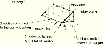
To create singular fields, 20-node bricks and 27-node bricks can be used with a collapsed face (see Figure 11.4.2–3).
The planes of the three-dimensional elements perpendicular to the crack line should be planar for the best accuracy. If they are not planar, the element Jacobian may become negative at some integration points when the midside nodes are moved to the 1/4 points. To correct this problem, move the midside nodes slightly away from the 1/4 points toward the midpoint position (the distance moved is not critical).See “Meshing the crack region and assigning elements,” Section 20.1.7 of the ABAQUS/CAE User's Manual, for information on creating a three-dimensional fracture mechanics mesh in ABAQUS/CAE.
To obtain a square root singularity, constrain the nodes on the collapsed face of the edge planes to move together and move the nodes to the 1/4 points.
If the nodes at the midplane of a collapsed 20-node brick are constrained to move together, ![]() ; therefore, the singularity is not the same on the midplane as on an edge plane. This difference causes local oscillations in the solution about the crack tip along the crack line, although normally the oscillations are not significant.
; therefore, the singularity is not the same on the midplane as on an edge plane. This difference causes local oscillations in the solution about the crack tip along the crack line, although normally the oscillations are not significant.
If all midface nodes and the centroid node are included in a 27-node brick and the midside and midface nodes are moved to the 1/4 points closest to the crack line, the oscillation in the local stress and strain fields can be reduced.
| Input File Usage: | *NFILL, SINGULAR |
Constrain the collapsed nodes to move together by specifying the same node number in the list of nodes forming the element or by using a linear constraint equation or multi-point constraint to tie them together. |
| ABAQUS/CAE Usage: | Interaction module: Special |
To obtain a ![]() singularity, allow the three nodes on the collapsed face to displace independently and keep the midside nodes at the midpoints.
singularity, allow the three nodes on the collapsed face to displace independently and keep the midside nodes at the midpoints.
| Input File Usage: | *NFILL |
| ABAQUS/CAE Usage: | Interaction module: Special |
To obtain a combined square root and ![]() singularity, allow the nodes on the collapsed face to displace independently and move the midside nodes to the 1/4 points. As in the two-dimensional case, if it is difficult to create the mesh with the nodes moved to the 1/4 points, simply use the
singularity, allow the nodes on the collapsed face to displace independently and move the midside nodes to the 1/4 points. As in the two-dimensional case, if it is difficult to create the mesh with the nodes moved to the 1/4 points, simply use the ![]() singularity.
singularity.
| Input File Usage: | *NFILL, SINGULAR |
| ABAQUS/CAE Usage: | Interaction module: Special |
The size of the crack-tip elements influences the accuracy of the solutions: the smaller the radial dimension of the elements from the crack tip, the better the stress, strain, etc. results will be and, therefore, the better the contour integral calculations will be.
The angular strain dependence is not modeled with the singular elements. Reasonable results are obtained if typical elements around the crack tip subtend angles in the range of 10° (accurate) to 22.5° (moderately accurate).
Since the crack tip causes a stress concentration, the stress and strain gradients are large as the crack tip is approached. Path dependence in the evaluation of the J-integral may be an indication that the mesh is not sufficiently refined, but path independence does not prove mesh convergence. The finite element mesh must be refined in the vicinity of the crack to get accurate stresses and strains; however, accurate J-integral results can frequently be obtained even with a relatively coarse mesh.
In many cases if sufficiently fine meshes are used, accurate contour integral values can be obtained without using singular elements.
Focused meshes can be used, but not all of the three-dimensional shell elements in ABAQUS/Standard can be collapsed. Elements S8R and S8RT cannot be degenerated into triangles; element types S4, S4R, S4R5, S8R5, and S9R5 can.
The quarter-point technique (moving the midside nodes to the quarter points to give a ![]() singularity for elastic fracture mechanics applications) can be used with S8R5 and S9R5 elements but not with S8R(T) elements. When the quarter-point technique is used with S9R5 elements, the midface node should be moved to the quarter-point position along with the two midside nodes.
singularity for elastic fracture mechanics applications) can be used with S8R5 and S9R5 elements but not with S8R(T) elements. When the quarter-point technique is used with S9R5 elements, the midface node should be moved to the quarter-point position along with the two midside nodes.
If S8R(T) elements are used, a keyhole should be introduced at the crack tip.
Flaws lying in the plane through the thickness of a shell can be modeled using line spring elements; see “Line spring elements for modeling part-through cracks in shells,” Section 26.10.1. In many cases line spring elements provide accurate J-integral and stress intensity values, but these elements are limited to modeling small strain and rotations. Limited modeling of plasticity is also allowed with line springs.
In large-strain analysis (when geometric nonlinearities are included) singular elements should not normally be used. The mesh must be sufficiently refined to model the very high strain gradients around the crack tip if details in this region are required. Even if only the J-integral is required, the deformation around the crack tip may dominate the solution and the crack-tip region will have to be modeled with sufficient detail to avoid numerical problems.
Physically, the crack tip is not perfectly sharp. Therefore, it is normally modeled as a blunted notch with a radius of ![]() , where
, where ![]() is a characteristic dimension of the plastic zone ahead of the crack tip. The notch must be small enough that, at the loads of interest, the deformed shape of the notch no longer depends on the original geometry. Typically, the notch must blunt out to more than four times its original radius for the deformed shape to be independent of the original geometry. The size of the elements around the notch should be about 1/10 the notch-tip radius to obtain accurate results.
is a characteristic dimension of the plastic zone ahead of the crack tip. The notch must be small enough that, at the loads of interest, the deformed shape of the notch no longer depends on the original geometry. Typically, the notch must blunt out to more than four times its original radius for the deformed shape to be independent of the original geometry. The size of the elements around the notch should be about 1/10 the notch-tip radius to obtain accurate results.
If a crack is modeled as sharp, the finite elements near the crack tip may not be able to approximate the high gradients, resulting in convergence problems. The stress and strain results around the crack tip will probably be inaccurate even if convergence is achieved. However, if the solution converges, the contour integral results should be reasonably accurate. The convergence difficulties will probably be greater in three dimensions than in two dimensions.
In situations involving finite rotations but small strains, such as bending of slender structures, a small “keyhole” around the crack tip should be modeled. If the hole is small, the results will not be affected significantly and problems in dealing with the singular strains at the crack tip will be avoided.
General multi-point constraints and linear constraint equations (“Kinematic constraints: overview,” Section 28.1.1) should not be used on nodes in the mesh regions where contour integrals are calculated unless the nodes involved in the constraint are located at the same point. The nodes at the crack tip of a focused mesh can be tied together using multi-point constraints without adversely affecting the contour integral calculations. Tying these nodes will change the singularity at the crack tip, but path independence of the contour integral will be maintained. In addition, path independence of the contour integrals will not be affected if two faces of a model are joined using MPC type TIE or a linear constraint equation, provided that all nodes of the two faces are coincident. Using multi-point constraints for mesh refinement or for applying symmetry/antisymmetry boundary conditions within the contour integral region will result in path dependence of the contour integrals. No warning or error messages are provided if this rule is violated.
Contour integrals can be requested in fracture mechanics problems modeled using the following procedures:
static (“Static stress analysis,” Section 6.2.2);
quasi-static (“Quasi-static analysis,” Section 6.2.5);
steady-state transport (“Steady-state transport analysis,” Section 6.4.1);
coupled thermal-stress procedures (“Fully coupled thermal-stress analysis,” Section 6.5.4); and
crack propagation (“Crack propagation analysis,” Section 11.4.3).
Contour integrals can be requested only in general analysis steps: they are not calculated in linear perturbation analyses (“General and linear perturbation procedures,” Section 6.1.2).
Contour integral calculations include the following distributed load types:
thermal loads;
distributed loads, including crack face pressure loads on continuum elements as well as those applied using user subroutine DLOAD;
uniform and nonuniform body forces; and
centrifugal loads on continuum elements.
Contributions to the contour integral due to concentrated loads in the domain are not included; instead, the mesh must be modified to include a small element and a distributed load must be applied to this element.
Contributions due to contact forces are not included.
J-integral calculations are valid for linear elastic, nonlinear elastic, and elastic-plastic materials. Plastic behavior can be modeled as nonlinear elastic (“Deformation plasticity,” Section 18.2.13), but the results are generally best if the material is modeled by incremental plasticity and is subject to proportional, monotonic traction loading.
If unloading has taken place in the plastic zone around the crack tip, the J-integral will not be valid except in very limited cases.
The ![]() -integral is valid for problems involving creep (“Rate-dependent plasticity: creep and swelling,” Section 18.2.4).
-integral is valid for problems involving creep (“Rate-dependent plasticity: creep and swelling,” Section 18.2.4).
The stress intensity factor calculation is valid for cracks in homogeneous, linear elastic materials. It is also valid for an interfacial crack between two different isotropic linear elastic materials.
The crack propagation direction is valid only for homogeneous, isotropic linear elastic materials.
The T-stress is valid only for homogeneous, isotropic linear elastic materials. Although the T-stress is calculated using the linear elastic material properties of the body with a crack, it is usually used with the J-integral calculated using the elastic-plastic material properties of the body (see “T-stress extraction,” Section 2.16.3 of the ABAQUS Theory Manual).
The contour integral evaluation capability in ABAQUS/Standard assumes that the elements that lie within the domain used for the calculations are quadrilaterals in two-dimensional or shell models or bricks in continuum three-dimensional models. Triangles, tetrahedra, or wedges should not be used in the mesh that is included in the contour integral regions. When the elements around the crack tip are generated in ABAQUS/CAE, triangular elements (in two dimensions) or wedge elements (in three dimensions) are converted to collapsed quadrilateral or hexahedral elements. The elements within the contour domain should be of the same type.
In shell structures the contour integrals calculated by ABAQUS/Standard will be contour independent only if the deformation mode around the crack tip is primarily membrane. If there are significant bending or transverse shear effects in the domain, the contour integrals may not be contour independent and contour integral values should be obtained directly from the displacements and/or the stresses.
Generalized plane strain elements, generalized axisymmetric elements with twist, asymmetric-axisymmetric elements, membrane elements, and cylindrical elements should not be used in the contour integral regions.
The contribution of rebar is included only in the calculations of the J-integral and the ![]() -integral for shell elements defined with a shell section integrated during the analysis (see “Using a shell section integrated during the analysis to define the section behavior,” Section 23.6.5).
-integral for shell elements defined with a shell section integrated during the analysis (see “Using a shell section integrated during the analysis to define the section behavior,” Section 23.6.5).
The domain associated with each contour is calculated automatically. The nodes belonging to each domain can be printed in the data file; see “Controlling the amount of analysis input file processor information written to the data file” in “Output,” Section 4.1.1. For each domain ABAQUS/Standard will create a new node set in the output database to include these nodes; you can view these node sets in ABAQUS/CAE. New node sets will also be created in the output database for nodes on crack surfaces and on free surfaces whose nodal normals are calculated by ABAQUS/Standard. Contour integrals cannot be recovered from the restart file as described in “Output,” Section 4.1.1.
You should not request element output extrapolated to the nodes (“Element output” in “Output to the data and results files,” Section 4.1.2) for second-order elements with one collapsed side in two dimensions or one collapsed face in three dimensions.
By default, the contour integral values are written to the data file and to the output database file. The following naming convention is used for contour integrals written to the output database:
integral-type: abbrev-integral-type at history-output-request-name_crack-name_internal-crack-tip-node-set-name__Contour_contour-numberwhere integral-type can be
Crack propagation direction (Cpd)
J-integral (J)
J-integral estimated from Ks (JKs)
Stress intensity factor K1 (K1)
Stress intensity factor K2 (K2)
T-stress (T)
J-integral: J at JINT_CRACK_CRACKTIP-1__Contour_1
You can choose to write the contour integral values to the results file in addition to the data file.
| Input File Usage: | Use the following option to write the contour integrals to the results file instead of the data file: |
*CONTOUR INTEGRAL, CONTOURS=n, OUTPUT=FILE Use the following option to write the contour integrals to the results file in addition to the data file: *CONTOUR INTEGRAL, CONTOURS=n, OUTPUT=BOTH |
| ABAQUS/CAE Usage: | You cannot write contour integrals to the results file from ABAQUS/CAE. |
You can control the output frequency, in increments, of contour integrals. By default, the crack-tip location and associated quantities will be printed every increment. Specify an output frequency of 0 to suppress contour integral output.
The output frequency for contour integral output to the output database is controlled by the larger of the frequency values specified for history output to the output database (see “Output to the output database,” Section 4.1.3) or for contour integral output. If you specify an output frequency of 0 for the history output to the output database, contour integral values will not be written to the output database.
| Input File Usage: | *CONTOUR INTEGRAL, CRACK NAME=crack name, CONTOURS=n, FREQUENCY=f |
| ABAQUS/CAE Usage: | Step module: history output request editor: Domain: Contour integral name: crack name, Number of contours: n, Save output at |