Product: ABAQUS/Standard
The air cavity resonance in a tire is often a significant contributor to the vehicle interior noise, particularly when the resonance of the tire couples with the cavity resonance. The purpose of this example is to study the acoustic response of a tire and air cavity subjected to an inflation pressure and footprint load. This example further demonstrates how the *ADAPTIVE MESH option can be used to update an acoustic mesh when structural deformation causes significant changes to the geometry of the acoustic domain. The effect of rolling motion is ignored; however, the rolling speed can have a significant influence on the coupled acoustic-structural response. This effect is investigated in detail in “Dynamic analysis of an air-filled tire with rolling transport effects,” Section 3.1.9.
The acoustic elements in ABAQUS model only small-strain dilatational behavior through pressure degrees of freedom and, therefore, cannot model the deformation of the fluid when the bounding structure undergoes large deformation. ABAQUS solves the problem of computing the current configuration of the acoustic domain by periodically creating a new acoustic mesh. The new mesh uses the same topology (elements and connectivity) throughout the simulation, but the nodal locations are adjusted periodically so that the deformation of the structural-acoustic boundary does not lead to severe distortion of the acoustic elements. The calculation of the updated nodal locations is based on adaptive mesh smoothing.
A detailed description of the tire model is provided in “Symmetric results transfer for a static tire analysis,” Section 3.1.1. We model the rubber as an incompressible hyperelastic material and include damping in the structure by specifying a 1-term Prony series viscoelastic material model with a relaxation modulus of 0.3 and relaxation time of 0.1 s. We define the model in the frequency domain using the *VISCOELASTIC, FREQUENCY=PRONY option since we want to include the damping effects in a steady-state dynamics simulation.
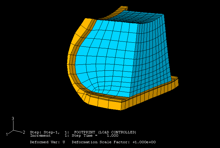
The air cavity in the model is defined as the space enclosed between the interior surface of the tire and a cylindrical surface of the same diameter as the diameter of the bead. A segment of the tire is shown in Figure 3.1.5–1. The values of the bulk modulus and the density of air are taken to be 426 kPa and 3.6 kg/m3, respectively, and represent the properties of air at the tire inflation pressure.
The simulation assumes that both the road and rim are rigid. We further assume that the contact between the road and the tire is frictionless during the preloading analyses. However, we use a nonzero friction coefficient in the subsequent coupled acoustic-structural analyses.
We use a tire model that is identical to that used in the simulation described in “Symmetric results transfer for a static tire analysis,” Section 3.1.1. The air cavity is discretized using linear acoustic elements and is coupled to the structural mesh using the *TIE option with the slave surface defined on the acoustic domain. We model the rigid rim by applying fixed boundary conditions to the nodes on the bead of the tire, while the interaction between the air cavity and rim is modeled by a traction-free surface; i.e., no boundary conditions are prescribed on the surface.
The *SYMMETRIC MODEL GENERATION and *SYMMETRIC RESULTS TRANSFER options, together with a *STATIC analysis procedure, are used to generate the preloading solution, which serves as the base state in the subsequent coupled acoustic-structural analyses.
In the first coupled analysis we compute the eigenvalues of the tire and air cavity system. This analysis is followed by a direct and a subspace projection steady-state dynamics analysis in which we obtain the response of the tire-air system subjected to harmonic excitation of the spindle.
A coupled structural-acoustic substructure analysis is performed as well. Viscoelasticity material is ignored in this simulation since the only form of damping the substructure can accurately represent is Raleigh-type damping. The substructure is generated by retaining 50 eigenmodes and the structural degrees of freedom at only two nodes: the road reference node and the wheel spindle. An equivalent model without substructures is also included and serves as reference solution.
The loading sequence for computing the footprint solution is identical to that discussed in “Symmetric results transfer for a static tire analysis,” Section 3.1.1. The simulation starts with an axisymmetric model, which includes the mesh for the air cavity. Only half the cross-section is modeled. The inflation pressure is applied to the structure using a *STATIC analysis. In this example the application of pressure does not cause significant changes to the geometry of the air cavity, so it is not necessary to update the acoustic mesh. However, we perform adaptive mesh smoothing after the pressure is applied to illustrate that the updated geometry of the acoustic domain is transferred to the three-dimensional model when symmetric results transfer is used.
The axisymmetric analysis is followed by a partial three-dimensional analysis in which the footprint solution is obtained. The footprint load is established over several load increments. The deformation during each load increment causes significant changes to the geometry of the air cavity. We update the acoustic mesh by performing 5 mesh sweeps after each converged structural load increment using the *ADAPTIVE MESH option. At the end of this analysis sequence we activate friction between the tire and road using the *CHANGE FRICTION option. This footprint solution, which includes the updated acoustic domain, is transferred to a full three-dimensional model. This model is used to perform the coupled analysis. In the first coupled analysis we extract the eigenvalues of the undamped system, followed by a *STEADY STATE DYNAMICS, DIRECT analysis in which we apply a harmonic excitation to the reference node of the rigid surface that is used to model the road. We perform two simulations: one in which the excitation is applied normal to the road surface and one in which the excitation is applied parallel to the road surface along the rolling (fore-aft) direction.
We want to compute the response of the coupled system in the frequency range in which we expect the air cavity to contribute to the overall acoustic response. We consider the response near the first eigenfrequency of the air cavity only, which has a wavelength that is equal to the circumference of the tire. Using a value of 344 m/s for the speed of sound and an air cavity radius of 0.240 m (the average of the minimum and maximum radius of the air cavity), we estimate this frequency to be approximately 230 Hz. We extract the eigenvalues and perform the steady-state dynamic analysis in the frequency range between 200 Hz to 260 Hz. Stiffness contributions from the frequency-dependent viscoelasticity material model are evaluated at a frequency of 230 Hz in the eigenvalue analysis. The PROPERTY EVALUATION parameter on the *FREQUENCY option is used for this purpose.
The same inflation and loading steps were used for the substructure analysis. The model is forced up and down by a *BOUNDARY condition specified at the road reference node in the *STEADY STATE DYNAMICS, DIRECT step and by an equivalent secondary *BASE MOTION in the *STEADY STATE DYNAMICS, SUBSPACE PROJECTION step. The INTERVAL=RANGE parameter on the *STEADY STATE DYNAMICS option is used to avoid computing unbounded responses at eigenfrequencies.
Figure 3.1.5–1 shows the updated acoustic mesh near the footprint region. The geometric changes associated with the updated mesh are taken into account in the coupled acoustic-structural analyses.
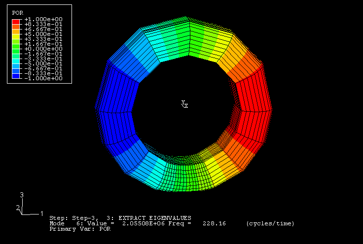
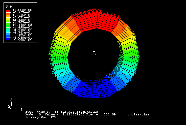
The eigenvalues of the air cavity, the tire, and the coupled tire-air system are tabulated in Table 3.1.5–1. The resonant frequencies of the uncoupled air cavity are computed using the original configuration. We obtain two acoustic modes at frequencies of 227.98 Hz and 230.17 Hz. These frequencies correspond to two identical modes rotated 90° with respect to each other, as shown in Figure 3.1.5–2 and Figure 3.1.5–3; the magnitudes of the frequencies are different since we have used a nonuniform mesh along the circumferential direction. We refer to the two modes as the fore-aft mode and the vertical mode, respectively. These eigenfrequencies correspond very closely to our original estimate of 230 Hz. The table shows that these eigenfrequencies occur at almost the same magnitude in the coupled system, indicating that the coupling has a very small effect on the acoustic resonance. The difference between the two vertical modes is larger than the difference between the fore-aft modes. This can be attributed to the geometry changes associated with structural loading. The coupling has a much stronger influence on the structural modes than on the acoustic modes, but we expect the coupling to decrease as we move away from the 230 Hz range.
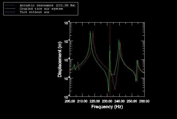
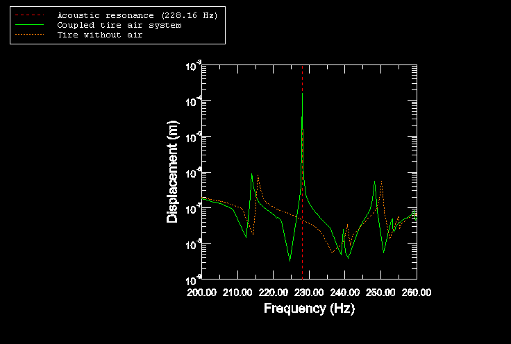
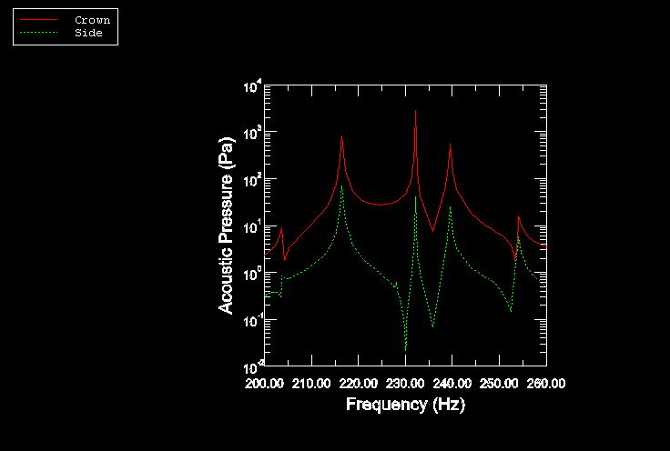
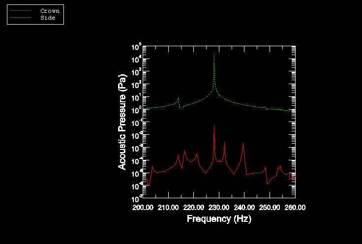
Figure 3.1.5–4 to Figure 3.1.5–7 show the response of the structure to the spindle excitation. Figure 3.1.5–4 and Figure 3.1.5–5 compare the response of the coupled tire-air system to the response of a tire without the air cavity. Figure 3.1.5–6 and Figure 3.1.5–7 show the acoustic pressure measured in the crown and side of the air. We draw the following conclusions from these figures. The frequencies at which resonance is predicted by the steady-state dynamic analysis correspond closely to the eigenfrequencies. However, not all the eigenmodes are excited by the spindle excitations. For example, the fore-aft mode is not excited by vertical loading. Similarly, the vertical mode is not excited by fore-aft loading. In addition, only some of the structural modes are excited by the spindle loads, while others are suppressed by material damping. These figures further show that the air cavity resonance has a very strong influence on the behavior of the coupled system and that the structural resonance of the coupled tire-air system occurs at different frequencies than the resonance of the tire without air. As expected, this coupling effect decreases as we move further away from the cavity resonance frequency.
The eigenfrequencies obtained in the substructure analysis are identical to the eigenfrequencies obtained in the equivalent analysis without substructures. The reaction force obtained at the road reference node is also compared to the reaction force at the same node in the equivalent analysis without substructures. As shown in Figure 3.1.5–8 the results for the two *STEADY STATE DYNAMICS steps in the substructure analysis are virtually identical, and they compare well, in general, with the reaction force obtained in the nonsubstructure analysis. The observed differences are due to the fact that only a relatively small number of eigenmodes are used to generate the substructure; and, hence, the dynamics of the substructure are not fully captured. Moreover, since there is no damping in these models (viscoelastic material effects are ignored), the response at eigenfrequencies is infinite. Consequently, the reaction forces are less predictable near eigenfrequencies, which explains some of the differences near the peaks.
Axisymmetric model, inflation analysis.
Partial three-dimensional model, footprint analysis.
Full three-dimensional model, coupled structural-acoustic analyses.
Nodal coordinates for the axisymmetric tire mesh.
Mesh data for the axisymmetric acoustic mesh.
Axisymmetric model, inflation analysis, no viscoelasticity.
Partial three-dimensional model, footprint analysis, no viscoelasticity.
Full three-dimensional model, coupled structural-acoustic analyses, no viscoelasticity, static analysis only.
Full three-dimensional model, coupled structural-acoustic analyses, no viscoelasticity, no substructures, *FREQUENCY and *STEADY STATE DYNAMICS analyses.
Full three-dimensional model, coupled structural-acoustic analyses, no viscoelasticity, substructure generation analysis.
Substructure usage analysis (*FREQUENCY and *STEADY STATE DYNAMICS analyses).