Product: ABAQUS/Standard
This example extends the analyses of “Coupled acoustic-structural analysis of a tire filled with air,” Section 3.1.5, to include rolling transport effects in the tire and air. The acoustic cavity is modeled as part of an axisymmetric model, which is inflated, revolved, reflected, and deformed to obtain a footprint in a manner consistent with the aforementioned example.
The purpose of this example is to examine the effect of steady-state rolling transport on the acoustic response of the tire and air cavity, after it has been subjected to the inflation pressure and footprint load. The air cavity resonance in a tire is often a significant contributor to the vehicle interior noise, particularly when the resonance of the tire couples with the cavity resonance. This coupled resonance phenomenon, however, is affected by the rotating motion in the fluid and the solid.
A detailed description of the tire model is provided in “Symmetric results transfer for a static tire analysis,” Section 3.1.1. We model the rubber as an incompressible hyperelastic material. Viscoelasticity in the material is ignored in this example.
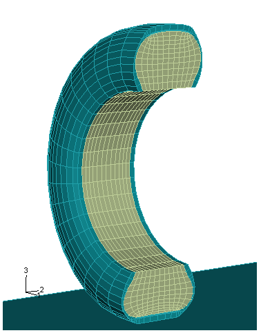
The air cavity in the model is defined as the space enclosed between the interior surface of the tire and a cylindrical surface of the same diameter as the diameter of the bead. A cross-section of the tire model is shown in Figure 3.1.9–1. The values of the bulk modulus and the density of air are taken to be 426 kPa and 3.6 kg/m3, respectively, and represent the properties of air at the tire inflation pressure.
The simulation assumes that both the road and rim are rigid. We further assume that the contact between the road and the tire is frictionless during the preloading analyses. However, we use a nonzero friction coefficient in the subsequent coupled acoustic-structural analyses.
To assess the effect of rolling motion on the dynamics of the coupled tire-air system, we first generate dynamic results for the stationary tire. In a subsequent analysis the tire and air are set into rolling motion, and corresponding dynamic results are obtained. In this analysis we also bring the air to rest while the tire is still in motion to assess the relative effect of the solid medium's motion alone.
We use a tire model that is identical to that used in the simulation described in “Symmetric results transfer for a static tire analysis,” Section 3.1.1. The air cavity is discretized using linear acoustic elements and is coupled to the structural mesh using the *TIE option with the slave surface defined on the acoustic domain. We model the rigid rim by applying fixed boundary conditions to the nodes on the bead of the tire, while the interaction between the air cavity and rim is modeled by a traction-free surface; i.e., no boundary conditions are prescribed on the surface.
We first create an axisymmetric mesh of half of the cross-section of the tire and air, then revolve it into half-symmetry. The *SYMMETRIC MODEL GENERATION and *SYMMETRIC RESULTS TRANSFER options, together with a *STATIC analysis procedure, are used to generate the preloading solution, which serves as the base state in the subsequent coupled acoustic-structural analyses.
In the first coupled analysis we reflect the revolved tire and air model into a full three-dimensional configuration. We then compute the real eigenvalues of the stationary tire and air cavity system. During frequency extraction steps, we impose fixed boundary conditions on the tire-road interface. This analysis is followed by a direct steady-state dynamic analysis in which we obtain the response of the tire-air system subjected to imposed harmonic motion of the spindle. Complex frequencies are also computed in this coupled analysis.
In the second coupled analysis the reflected model is restarted from the first step, after the footprint equilibrium configuration had been established. The *STEADY STATE TRANSPORT option is used to compute the rolling equilibrium state in the solid material, via the *TRANSPORT VELOCITY option, corresponding to a speed of roughly 80 km/hr. In this step the *ACOUSTIC FLOW VELOCITY option signifies that the acoustic medium is also in rotational motion. The direct steady-state analysis, with similar parameters to those used in the stationary case, is repeated. Finally, the air is brought to rest while the tire is still in motion to separate the relative contributions of the rolling tire and air, and the steady-state dynamics results are repeated.
The loading sequence for computing the footprint solution is identical to that discussed in “Symmetric results transfer for a static tire analysis,” Section 3.1.1. The simulation starts with an axisymmetric model, which includes the mesh for the air cavity. Only half the cross-section is modeled. The inflation pressure is applied to the structure using a *STATIC analysis. In this example the application of pressure does not cause significant changes to the geometry of the air cavity, so it is not necessary to update the acoustic mesh. However, we perform adaptive mesh smoothing after the pressure is applied to illustrate that the updated geometry of the acoustic domain is transferred to the three-dimensional model when symmetric results transfer is used.
The axisymmetric analysis is followed by a reflection—symmetric three-dimensional analysis in which the footprint solution is obtained. The footprint load is established over several load increments. The deformation during each load increment causes significant changes to the geometry of the air cavity. We update the acoustic mesh by performing five mesh sweeps after each converged structural load increment using the *ADAPTIVE MESH option. At the end of this analysis sequence we activate friction between the tire and road using the *CHANGE FRICTION option. This footprint solution, which includes the updated acoustic domain, is transferred to a full three-dimensional model. This model is used to perform the coupled analysis. In the first coupled analysis we extract the eigenvalues of the undamped system, followed by a *STEADY STATE DYNAMICS, DIRECT analysis in which we apply a harmonic excitation to the reference node of the rigid surface that is used to model the road.
In the stationary and rolling analyses we compute the response of the coupled system in the same frequency range used in “Coupled acoustic-structural analysis of a tire filled with air,” Section 3.1.5 (200 to 260 Hz). This band includes the natural frequency of one stationary acoustic-only mode, at roughly 230 Hz.
The same inflation and loading steps are used for the substructure analysis. The model is forced up and down by a *BOUNDARY condition specified at the road reference node in the *STEADY STATE DYNAMICS, DIRECT step and by an equivalent secondary *BASE MOTION in the *STEADY STATE DYNAMICS, SUBSPACE PROJECTION step. The INTERVAL=RANGE parameter on the *STEADY STATE DYNAMICS option is used to avoid computing unbounded responses at eigenfrequencies.
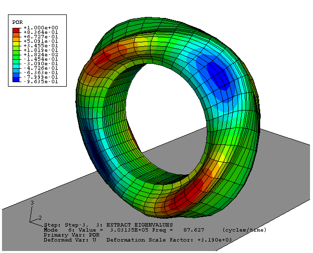
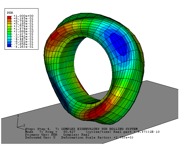
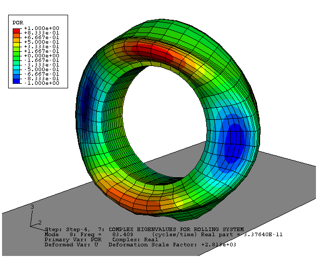
The characteristic frequencies of the coupled tire-air system are affected by the rolling motion. Generally, we expect a mode observed in the stationary coupled tire-air system to convert to a pair of modes, corresponding to forward and backward wave travel. This does not always occur in complex systems, because the stationary modes are not all affected by the rolling motion to a similar degree. The resonant frequencies of the stationary case are computed using the real-valued frequency extraction procedure (*FREQUENCY), although the complex frequency procedure will yield identical results for the stationary case. For the rolling analysis the complex frequency procedure must be used to obtain accurate results using all of the element contributions due to motion. The real parts of these eigenvalues are, however, nearly zero in this case because no damping is applied in the problem. In Table 3.1.9–1 an example is shown of a stationary mode splitting into a pair of modes in the rolling case. The modes are shown in Figure 3.1.9–2, Figure 3.1.9–3, and Figure 3.1.9–4. Because the footprint nodes are fixed in this example, the resonant frequencies for the stationary case are different than those computed in “Coupled acoustic-structural analysis of a tire filled with air,” Section 3.1.5.
Figure 3.1.9–5, Figure 3.1.9–6, and Figure 3.1.9–7 show the response of the structure to the imposed vertical motion at the spindle. Figure 3.1.9–5 compares the acoustic response, at the crown, of the coupled tire-air system for the stationary, full rolling at 80 km/hr, and solid rolling cases. Figure 3.1.9–6 is a similar frequency response diagram for the acoustic pressure at the side of the tire, and Figure 3.1.9–7 shows the vertical reaction force.
The frequencies at which resonance is predicted by the steady-state dynamic analyses at stationary and air/solid rolling correspond closely to the eigenfrequencies predicted in these cases (see Table 3.1.9–2). However, not all the eigenmodes are excited by the spindle excitations. These figures further show that the rolling motion of the solid has a very strong influence on the behavior of the coupled system and that the rolling motion of the air exerts a similarly strong effect in the frequency range observed here. In particular, the resonances affecting the reaction force occur at different frequencies for the stationary, solid rolling, and air/solid rolling cases. The resonances observed in the reaction force frequency response diagram also proliferate as rolling is introduced since waves traveling against and with the direction of rolling propagate at different speeds with respect to the observer.
Axisymmetric model, inflation analysis.
Partial three-dimensional model, footprint analysis.
Full three-dimensional model, coupled structural-acoustic analyses, no transport effects.
Full three-dimensional model, coupled structural-acoustic analyses, transport effects at moderate speed.
Nodal coordinates for the axisymmetric tire mesh.
Mesh data for the axisymmetric acoustic mesh.
Table 3.1.9–1 Example of eigenvalue splitting.
| Mode description | Stationary coupled air-tire | Rolling coupled air-tire |
|---|---|---|
| coupled, 2-lobe | 87.627 (#6) | 80.427 (#7), 83.409 (#8) |
Table 3.1.9–2 Eigenvalues in rolling state between 200 and 230 Hz.
| Mode | No motion | Solid only in motion | Solid and air in motion |
|---|---|---|---|
| 1 | 202.70 | 202.18 | 202.20 |
| 2 | 204.69 | 205.69 | 207.66 |
| 3 | 207.04 | 209.60 | 210.30 |
| 4 | 211.83 | 210.87 | 214.04 |
| 5 | 214.17 | 215.69 | 214.66 |
| 6 | 216.72 | 215.93 | 214.89 |
| 7 | 217.08 | 219.99 | 216.82 |
| 8 | 223.85 | 223.76 | 216.83 |
| 9 | 224.67 | 225.38 | 221.42 |
| 10 | 225.81 | 225.98 | 224.81 |
| 11 | 227.62 | 227.63 | 227.54 |
| 12 | 228.81 | 230.32 | (241.67) |