Product: ABAQUS/Standard
This example illustrates the use of the *SYMMETRIC RESULTS TRANSFER option as well as the *SYMMETRIC MODEL GENERATION option to model the static interaction between a tire and a rigid surface.
The *SYMMETRIC MODEL GENERATION option (“Symmetric model generation,” Section 10.3.1 of the ABAQUS Analysis User's Manual) can be used to create a three-dimensional model by revolving an axisymmetric model about its axis of revolution or by combining two parts of a symmetric model, where one part is the original model and the other part is the original model reflected through a line or a plane. Both model generation techniques are demonstrated in this example.
The *SYMMETRIC RESULTS TRANSFER option (“Transferring results from a symmetric mesh or a partial three-dimensional mesh to a full three-dimensional mesh,” Section 10.3.2 of the ABAQUS Analysis User's Manual) allows the user to transfer the solution obtained from an axisymmetric analysis onto a three-dimensional model with the same geometry. It also allows the transfer of a symmetric three-dimensional solution to a full three-dimensional model. Both these results transfer features are demonstrated in this example. The results transfer capability can significantly reduce the analysis cost of structures that undergo symmetric deformation followed by nonsymmetric deformation later during the loading history.
The purpose of this example is to obtain the footprint solution of a 175 SR14 tire in contact with a flat rigid surface, subjected to an inflation pressure and a concentrated load on the axle. Input files modeling a tire in contact with a rigid drum are also included. These footprint solutions are used as the starting point in “Steady-state rolling analysis of a tire,” Section 3.1.2, where the free rolling state of the tire rolling at 10 km/h is determined and in “Subspace-based steady-state dynamic tire analysis,” Section 3.1.3, where a frequency response analysis is performed.
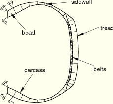
The different components of the tire are shown in Figure 3.1.1–1. The tread and sidewalls are made of rubber, and the belts and carcass are constructed from fiber-reinforced rubber composites. The rubber is modeled as an incompressible hyperelastic material, and the fiber reinforcement is modeled as a linear elastic material. A small amount of skew symmetry is present in the geometry of the tire due to the placement and ![]() 20.0° orientation of the reinforcing belts.
20.0° orientation of the reinforcing belts.
Two simulations are performed in this example. The first simulation exploits the symmetry in the tire model and utilizes the results transfer capability; the second simulation does not use the results transfer capability. Comparisons between the two methodologies are made for the case where the tire is in contact with a flat rigid surface. Input files modeling a tire in contact with a rigid drum are also included. The methodology used in the first analysis is applied in this simulation. Results for this case are presented in “Steady-state rolling analysis of a tire,” Section 3.1.2.
The first simulation is broken down into three separate analyses. In the first analysis the inflation of the tire by a uniform internal pressure is modeled. Due to the anisotropic nature of the tire construction, the inflation loading gives rise to a circumferential component of deformation. The resulting stress field is fully three-dimensional, but the problem remains axisymmetric in the sense that the solution does not vary as a function of position along the circumference. ABAQUS provides axisymmetric elements with twist (CGAX) for such situations. These elements are used to model the inflation loading. Only half the tire cross-section is needed for the inflation analysis due to a reflection symmetry through the vertical line that passes through the tire axle (see Figure 3.1.1–2). We refer to this model as the axisymmetric model.
The second part of the simulation entails the computation of the footprint solution, which represents the static deformed shape of the pressurized tire due to a vertical dead load (modeling the weight of a vehicle). A three-dimensional model is needed for this analysis. The finite element mesh for this model is obtained by revolving the axisymmetric cross-section about the axis of revolution. A nonuniform discretization along the circumference is used as shown in Figure 3.1.1–3. In addition, the axisymmetric solution is transferred to the new mesh where it serves as the initial or base state in the footprint calculations. As with the axisymmetric model, only half of the cross-section is needed in this simulation, but skew-symmetric boundary conditions must be applied along the midplane of the cross-section to account for antisymmetric stresses that result from the inflation loading and the concentrated load on the axle. We refer to this model as the partial three-dimensional model.
In the last part of this analysis the footprint solution from the partial three-dimensional model is transferred to a full three-dimensional model and brought into equilibrium. This full three-dimensional model is used in the steady-state transport example that follows. The model is created by combining two parts of the partial three-dimensional model, where one part is the mesh used in the second analysis and the other part is the partial model reflected through a line. We refer to this model as the full three-dimensional model.
A second simulation is performed in which the same loading steps are repeated, except that the full three-dimensional model is used for the entire analysis. Besides being used to validate the results transfer solution, this second simulation allows us to demonstrate the computational advantage afforded by the ABAQUS results transfer capability in problems with rotational and/or reflection symmetries.
In the first simulation the inflation step is performed on the axisymmetric model and the results are stored in the results files (.res, .mdl, .stt, and .prt). The axisymmetric model is discretized with CGAX4H and CGAX3H elements. The belts and ply are modeled with rebar in surface elements embedded in continuum elements. The ROUNDOFF TOLERANCE parameter on the *EMBEDDED ELEMENT option is used to adjust the positions of embedded element nodes such that they lie exactly on host element edges. This feature is useful in cases where embedded nodes are offset from host element edges by a small distance caused by numerical roundoff. Eliminating such gaps reduces the number of constraint equations used to embed the surface elements and, hence, improves performance. The axisymmetric results are read into the subsequent footprint analysis, and the partial three-dimensional model is generated by ABAQUS by revolving the axisymmetric model cross-section about the rotational symmetry axis. The *SYMMETRIC MODEL GENERATION, REVOLVE option is used for this purpose. The partial three-dimensional model is composed of four sectors of CCL12H and CCL9H cylindrical elements covering an angle of 320°, with the rest of the tire divided into 16 sectors of C3D8H and C3D6H linear elements. The linear elements are used in the footprint region. The use of cylindrical elements is recommended for regions where it is possible to cover large sectors around the circumference with a small number of elements. In the footprint region, where the desired resolution of the contact patch dictates the number of elements to be used, it is more cost-effective to use linear elements. The road (or drum) is defined as an analytical rigid surface in the partial three-dimensional model. The results of the footprint analysis are read into the final equilibrium analysis, and the full three-dimensional model is generated by reflecting the partial three-dimensional model through a vertical line using the *SYMMETRIC MODEL GENERATION, REFLECT=LINE option. The line used in the reflection is the vertical line in the symmetry plane of the tire, which passes through the axis of rotation. The REFLECT=LINE parameter is used, as opposed to the REFLECT=PLANE parameter, to take into account the skew symmetry of the tire. The analytical rigid surface as defined in the partial three-dimensional model is transferred to the full model without change. The three-dimensional finite element mesh of the full model is shown in Figure 3.1.1–4.
In the second simulation a datacheck analysis is performed to write the axisymmetric model information to the results files. The full tire cross-section is meshed in this model. No analysis is needed. The axisymmetric model information is read in a subsequent run, and a full three-dimensional model is generated by ABAQUS by revolving the cross-section about the rotational symmetry axis. The *SYMMETRIC MODEL GENERATION, REVOLVE option is again used for this purpose. The road is defined in the full model. The three-dimensional finite element mesh of the full model is identical to the one generated in the first analysis. However, the inflation load and concentrated load on the axle are applied to the full model without making use of the results transfer capability.
The footprint calculations are performed with a friction coefficient of zero in anticipation of eventually performing a steady-state rolling analysis of the tire using the *STEADY STATE TRANSPORT option, as explained in “Steady-state rolling analysis of a tire,” Section 3.1.2.
Since the results from the static analyses performed in this example are used in a subsequent time-domain dynamic example, the input files contain the following features that would not ordinarily be included for purely static analyses:
The TRANSPORT parameter is included with the *SYMMETRIC MODEL GENERATION option to define streamlines in the model, which are needed by ABAQUS to perform streamline calculations during the *STEADY STATE TRANSPORT analysis in the next example problem. The TRANSPORT parameter is not required for any analysis type except *STEADY STATE TRANSPORT.
The hyperelastic material that models the rubber has a *VISCOELASTIC, TIME=PRONY option included. This enables us to model viscoelasticity in the steady-state transport example that follows. As a consequence of defining a time-domain viscoelastic material property, the *HYPERELASTIC option includes the LONG TERM parameter to indicate that the elastic properties defined on the associated data lines define the long-term behavior of the rubber. In addition, all *STATIC steps include the LONG TERM parameter to ensure that the static solutions are based upon the long-term elastic moduli.
As discussed in the previous sections, the loading on the tire is applied over several steps. In the first simulation the inflation of the tire to a pressure of 200.0 kPa is modeled using the axisymmetric tire model (tiretransfer_axi_half.inp) with a *STATIC analysis procedure. The results from this axisymmetric analysis are then transferred to the partial three-dimensional model (tiretransfer_symmetric.inp) in which the footprint solution is computed in two sequential *STATIC steps. The first of these static steps establishes the initial contact between the road and the tire by prescribing a vertical displacement of 0.02 m on the rigid body reference node. Since this is a static analysis, it is recommended that contact be established with a prescribed displacement, as opposed to a prescribed load, to avoid potential convergence difficulties that might arise due to unbalanced forces. The prescribed boundary condition is removed in the second static step, and a vertical load of ![]() 1.65 kN is applied to the rigid body reference node. The 1.65 kN load in the partial three-dimensional model represents a 3.3 kN load in the full three-dimensional model. The transfer of the results from the axisymmetric model to the partial three-dimensional model is accomplished by using the *SYMMETRIC RESULTS TRANSFER, REVOLVE option. Once the static footprint solution for the partial three-dimensional model has been established, the *SYMMETRIC RESULTS TRANSFER, REFLECT option is used to transfer the solution to the full three-dimensional model (tiretransfer_full.inp), where the footprint solution is brought into equilibrium in a single *STATIC increment. The results transfer sequence is illustrated in Figure 3.1.1–5.
1.65 kN is applied to the rigid body reference node. The 1.65 kN load in the partial three-dimensional model represents a 3.3 kN load in the full three-dimensional model. The transfer of the results from the axisymmetric model to the partial three-dimensional model is accomplished by using the *SYMMETRIC RESULTS TRANSFER, REVOLVE option. Once the static footprint solution for the partial three-dimensional model has been established, the *SYMMETRIC RESULTS TRANSFER, REFLECT option is used to transfer the solution to the full three-dimensional model (tiretransfer_full.inp), where the footprint solution is brought into equilibrium in a single *STATIC increment. The results transfer sequence is illustrated in Figure 3.1.1–5.
Boundary conditions and loads are not transferred with the *SYMMETRIC RESULTS TRANSFER option; they must be carefully redefined in the new analysis to match the loads and boundary conditions from the transferred solution. Due to numerical and modeling issues the element formulations for the two-dimensional and three-dimensional elements are not identical. As a result, there may be slight differences between the equilibrium solutions generated by the two- and three-dimensional models. In addition, small numerical differences may occur between the symmetric and full three-dimensional solutions because of the presence of symmetry boundary conditions in the symmetric model that are not used in the full model. Therefore, it is advised that in a results transfer simulation an initial step be performed where equilibrium is established between the transferred solution and loads that match the state of the model from which the results are transferred. It is recommended that an initial *STATIC step with the initial time increment set to the total step time be used to allow ABAQUS/Standard to find the equilibrium in one increment.
In the second simulation identical inflation and footprint steps are repeated. The only difference is that the entire analysis is performed on the full three-dimensional model (tiretransfer_full_footprint.inp). The full three-dimensional model is generated using the restart information from a datacheck analysis of an axisymmetric model of the full tire cross-section (tiretransfer_axi_full.inp).
The default contact pair formulation in the normal direction is hard contact, which gives strict enforcement of contact constraints. Some analyses are conducted with both hard and augmented Lagrangian contact to demonstrate that the default penalty stiffness chosen by the code does not affect stress results significantly. The augmented Lagrangian method is invoked by specifying the AUGMENTED LAGRANGE parameter on the *SURFACE BEHAVIOR option. The hard and augmented Lagrangian contact algorithms are described in “Constraint enforcement methods for ABAQUS/Standard contact pairs,” Section 29.2.3 of the ABAQUS Analysis User's Manual.
Since the three-dimensional tire model has a small loaded area and, thus, rather localized forces, the default averaged flux values for the convergence criteria produce very tight tolerances and cause more iteration than is necessary for an accurate solution. To decrease the computational time required for the analysis, the *CONTROLS option can be used to override the default values for average forces and moments. The default controls are used in this example.
The results from the first two simulations are essentially identical. The peak Mises stresses and displacement magnitudes in the two models agree within 0.3% and 0.2%, respectively. The final deformed shape of the tire is shown in Figure 3.1.1–6. The computational cost of each simulation is shown in Table 3.1.1–1. The simulation performed on the full three-dimensional model takes 2.5 times longer than the results transfer simulation, clearly demonstrating the computational advantage that can be attained by exploiting the symmetry in the model using the *SYMMETRIC RESULTS TRANSFER option.
Axisymmetric model, inflation analysis (simulation 1).
Partial three-dimensional model, footprint analysis (simulation 1).
Partial three-dimensional model, footprint analysis using augmented Lagrangian contact (simulation 1).
Full three-dimensional model, final equilibrium analysis (simulation 1).
Full three-dimensional model, final equilibrium analysis using augmented Lagrangian contact (simulation 1).
Axisymmetric model, datacheck analysis (simulation 2).
Full three-dimensional model, complete analysis (simulation 2).
Partial three-dimensional model of a tire in contact with a rigid drum.
Full three-dimensional model of a tire in contact with a rigid drum.
Nodal coordinates for the axisymmetric models.
Axisymmetric model, inflation analysis (simulation 1) with Marlow hyperelastic model.
Partial three-dimensional model, footprint analysis (simulation 1) with Marlow hyperelastic model.
Full three-dimensional model, final equilibrium analysis (simulation 1) with Marlow hyperelastic model.
Table 3.1.1–1 Comparison of normalized CPU times for the footprint analysis (normalized with respect to the total “No results transfer” analysis).
| Use results transfer and symmetry conditions | No results transfer | |
|---|---|---|
| Inflation | 0.005(a)+0.040(b) | 0.347(e) |
| Footprint | 0.265(c)+0.058(d) | 0.653(e) |
| Total | 0.368 | 1.0 |
| (a) axisymmetric model | ||
| (b) equilibrium step in partial three-dimensional model | ||
| (c) footprint analysis in partial three-dimensional model | ||
| (d) equilibrium step in full three-dimensional model | ||
| (e) full three-dimensional model | ||