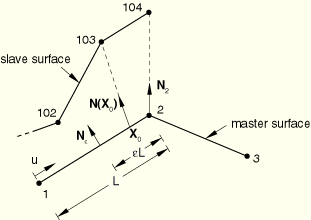
Although four internal element types are used to model the various types of small-sliding contact interactions supported by ABAQUS/Standard, all four formulations are based on the notion that a given slave node always interacts with the same subset of master surface nodes. This nodal subset is initially determined by the ABAQUS analysis input file processor from the undeformed model definition, thus avoiding the need to “track” the slave node during the course of the analysis. This set of nearest-neighbor nodes to the point on the master surface closest to the slave node is used to parametrize a contact plane with which the slave node will interact during the analysis. This concept is illustrated next for the case of a two-dimensional slave node interacting with a first-order master surface. This formulation can be generalized to second order as well as three-dimensional situations, but this generalization will not be discussed here.

Consider the contact interaction of three nodes—102, 103, and 104—on the slave surface with a master surface made up of first-order element faces described by nodes 1, 2, and 3, as shown in Figure 5.1.1–1.

Before initiating the search for the nodal subset of the master surface nodes that will interact with each node on the slave surface, unit normal vectors are computed for all the nodes on the master surface. For example, the unit normal vector is computed by averaging the unit normal vectors of segments 1–2 and 2–3. The user can also specify the normal vector for each node on the master surface. Additional unit normal vectors are computed for each segment a distance from each end of the segment, where is a fraction and is the length of the segment; e.g., . Currently the value of is set to 0.5, and the user cannot change this value. The unit normals computed are then used to define a smooth varying normal vector, , at any point, , on the master surface.

An “anchor” point on the master surface, , is computed for each slave node so that the vector formed by the slave node and coincides with the normal vector . Suppose that a search for the anchor point, , of slave node 103 reveals that is on segment 1–2. Then, we find that

where and are the coordinates of nodes 1 and 2, respectively, and is calculated so that coincides with . Moreover, the contact plane tangent direction, , at is chosen so that it is perpendicular to ; i.e., where is a (constant) rotation matrix.

The small-sliding contact constraint is achieved by requiring that slave node 103 interact with the tangent plane whose current anchor point coordinates are, at any time, given by

where and , and whose current tangent direction is given by where and . Since the above expressions for the point and the vector resulted from barycentric (affine) combinations of the points and —that is, the contact plane will be mapped properly under affine transformations such as translation, scaling (stretching), and rotation.

Next, suppose that a search for the anchor point of slave node 104 reveals that the anchor point is coincident to the master node 2. In this case the anchor point is chosen to be , or in terms of the coordinates of the three master nodes 1, 2, and 3,

where , , and . The contact tangent direction at is simply However, we want to express in terms of the coordinates of the three nodes 1, 2, and 3 to be able to track the evolution of the tangent plane. To this end, we solve for the from the equation subject to the barycentric constraint The barycentric constraint ensures that the resulting expression for the contact plane tangent direction behaves properly under affine transformations such as translations and rotations.

At each slave node that can come into contact with a master surface we construct a measure of overclosure (penetration of the node into the master surface) and measures of relative slip . These kinematic measures are then used, together with appropriate Lagrange multiplier techniques, to introduce surface interaction theories for contact and friction, as described in “Contact pressure definition,” Section 5.2.1, and “Coulomb friction,” Section 5.2.3.

In two dimensions the overclosure along the unit contact normal between a slave point and a master line , where parametrizes the line, is determined by finding the vector from the slave node to the line that is perpendicular to the tangent vector at . Mathematically, we express the required condition as

when

Similarly, in three dimensions the overclosure along the unit contact normal between a slave point and a master plane , where parametrize the plane, is determined by finding the vector from the slave node to the plane that is perpendicular to the tangent vectors and at . Mathematically, we express the required condition as

when

If at a given slave node , there is no contact between the surfaces at that node, and no further surface interaction calculations are needed. If , the surfaces are in contact. The contact constraint is enforced by introducing a Lagrange multiplier, , whose value provides the contact pressure at the point. To enforce the contact constraint, we need the first variation ; and for the Newton iterations, we need the second variation, . Likewise, if frictional forces are to be transmitted across the contacting surfaces, the first variations of relative slip, , and the second variations, , are needed in the formulation. The derivation of some of these quantities is described next for all four small-sliding contact formulations.

For the case of two-dimensional small-sliding deformable contact, a point on the contact line associated with a slave node is represented by the vector

where, as described previously, the line's anchor point——and its tangent vector——are functions of the current master node coordinates, . Hence, the vector is, in general, a nonunit vector. Linearization of Equation 5.1.1–1 yields where , , and .

Taking the dot product of Equation 5.1.1–4 with results in the following expression for :

Likewise, taking the dot product of Equation 5.1.1–4 with the normalized tangent vector and setting results in the following expression for the variation in slip:

Suitable expressions for and can be derived by linearizing Equation 5.1.1–4 and applying the techniques highlighted above. Since the resulting expressions do not provide additional insight into the understanding of this capability, they will not be presented here.

The three-dimensional small-sliding deformable contact formulation is a straightforward generalization of the previous two-dimensional formulation. A point on the contact plane associated with a slave node is represented by the vector

where the plane's anchor point——and its two tangent vectors— and —are functions of the current master node coordinates . Linearization of Equation 5.1.1–2 yields where and .

Taking the dot product of Equation 5.1.1–7 with results in the following expression for :

Likewise, taking the dot product of Equation 5.1.1–7 with and setting results in the following expression for the variation of the first slip component:

Similarly, taking the dot product of Equation 5.1.1–7 with and setting results in the following expression for the variation of the second slip component:

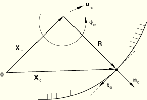
The formulation for two-dimensional small-sliding rigid contact follows from its deformable counterpart by exploiting the fact that the evolution of the contact plane is fully determined by the motion of the rigid body's reference node. Figure 5.1.1–2 shows how the undeformed coordinates of the contact plane's anchor point are related vectorially to the undeformed coordinates of the rigid reference node, , and the relative position vector .We can express this relationship as

Suppose the rigid reference node undergoes a motion described by the displacement vector and the rotation vector , then the current coordinates of the contact plane's anchor point are given by

where is the orthogonal matrix that produces the rotation (see “Rotation variables,” Section 1.3.1) and is the current position vector from the rigid reference node to the anchor point. The rotation matrix is also used to obtain the contact plane's current tangent and current normal as follows: where and are the initial contact tangent and normal at , respectively, as shown in Figure 5.1.1–2. By definition, a rigid surface cannot stretch; therefore, a point on the rigid contact line associated with a slave node is represented by the vector where—unlike the vector in Equation 5.1.1–3—the tangent is always a unit vector.

Linearization of Equation 5.1.1–11 and Equation 5.1.1–12 results in the following expressions for the first variations of the anchor coordinates and the contact plane's tangent:

Replacing by in Equation 5.1.1–5, noting that , and substituting for and from Equation 5.1.1–13 results in the following expression for :

Similar manipulation of Equation 5.1.1–6 yields the following expression for :

The three-dimensional small-sliding rigid contact formulation can also be derived from its deformable counterpart by generalizing some of the expressions that were introduced in the previous section. In particular, in this formulation the rigid reference node can undergo an arbitrary finite rotation described by the rotation vector . Consequently, Equation 5.1.1–13 for the variations of the anchor point coordinates and the contact plane's tangent generalize to

where is the skew-symmetric matrix associated with the linearized rotation , as explained in “Rotation variables,” Section 1.3.1.

Replacing by in Equation 5.1.1–8 through Equation 5.1.1–10 and substituting for and from above results in the following expressions for , , and :