Product: ABAQUS/Standard
ABAQUS/Standard provides two formulations for modeling the interaction between two deformable bodies. The first is a small-sliding formulation in which the contacting surfaces can undergo only relatively small sliding relative to each other but arbitrary rotation of the surfaces is permitted. This formulation is discussed in “Small-sliding interaction between bodies,” Section 5.1.1. The second is a finite-sliding formulation where separation and sliding of finite amplitude and arbitrary rotation of the surfaces may arise. The formulation for two-dimensional and axisymmetric analysis, as well as for tube-in-tube analysis, is discussed in this section.
Depending on the type of contact problem, two approaches are available to the user for specifying the finite-sliding capability: (1) defining possible contact conditions by identifying and pairing potential contact surfaces and (2) using contact elements. With the first approach ABAQUS automatically generates the appropriate contact elements.
In axisymmetric problems with asymmetric deformations, ISL21A and ISL22A elements can be used to model contact with CAXA or SAXA elements. Sliding of tubes inside each other can be modeled with ITT21 and ITT31 elements.
To define a sliding interface between two surfaces, one of the surfaces (the “slave” surface) is covered with ISL or ITT elements. The other surface (the “master” surface) is defined as a slide line surface composed of a series of nodes ordered in sequence. The slide line itself can consist of linear or quadratic segments. If smoothing is used, these segments are connected with quadratic or cubic segments such that full slope continuity is achieved. The smoothing procedure is described later in this section.
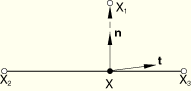
Consider contact of a node on the slave surface ![]() with a segment of the master surface described by nodes
with a segment of the master surface described by nodes ![]() ,
, ![]() ,
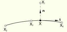
, ![]() , where the number of nodes depends on the order of the segment. For a linear segment the number of nodes is 2, whereas for a quadratic segment the number of nodes is 3. For a smoothed section of a linear slide line, the number of nodes is also 3; and for a smoothed section of a quadratic slide line, the number of nodes is 5. If the contact occurs at the (convex) vertex of two segments, only a single node will enter the equations. A typical linear segment is shown in Figure 5.1.2–1, and a quadratic segment is displayed in Figure 5.1.2–2. Smoothed segments are shown later in this section.
, where the number of nodes depends on the order of the segment. For a linear segment the number of nodes is 2, whereas for a quadratic segment the number of nodes is 3. For a smoothed section of a linear slide line, the number of nodes is also 3; and for a smoothed section of a quadratic slide line, the number of nodes is 5. If the contact occurs at the (convex) vertex of two segments, only a single node will enter the equations. A typical linear segment is shown in Figure 5.1.2–1, and a quadratic segment is displayed in Figure 5.1.2–2. Smoothed segments are shown later in this section.
To derive the equations governing these elements, we consider the coordinates in the plane of the slide line. For the axisymmetric elements, this plane coincides with the two-dimensional space. First, we determine the point ![]() on the segment closest to the point
on the segment closest to the point ![]() on the slave surface. We also determine the normal
on the slave surface. We also determine the normal ![]() and tangent
and tangent ![]() to the segment at that point. The point
to the segment at that point. The point ![]() and the normal
and the normal ![]() can be related to the overclosure
can be related to the overclosure ![]() with the relation
with the relation
![]()
![]()
To obtain the contact/slip equation, the position equation (Equation 5.1.2–2) is linearized. This linearization yields
![]()
![]()
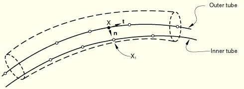
In the case of tube-tube interface elements it is assumed that the inner tube can be considered the slave surface and the outer tube the master surface. The tube-tube interface elements differ from the axisymmetric slide line elements in two ways. In the first place there is assumed to be a finite clearance between the tubes, which has the effect that the separation distance ![]() is finite even when contact occurs. In the second place for the three-dimensional element ITT31 there is a second possible slip direction in the plane of the cross-section of the tubes. The derivations for the ITT elements follow much along the same line as the derivations for the ISL elements. The contact equation can be written in the form
is finite even when contact occurs. In the second place for the three-dimensional element ITT31 there is a second possible slip direction in the plane of the cross-section of the tubes. The derivations for the ITT elements follow much along the same line as the derivations for the ISL elements. The contact equation can be written in the form
In this equation ![]() is the (positive) radial clearance between the tubes. In a similar way as was done for the ISL elements, the contact equation can be written in the form
is the (positive) radial clearance between the tubes. In a similar way as was done for the ISL elements, the contact equation can be written in the form
![]()
The initial stress stiffness terms are again obtained by taking the second variations in ![]() ,
, ![]() , and
, and ![]() . From Equation 5.1.2–17 follows
. From Equation 5.1.2–17 follows
Substitution of Equation 5.1.2–20 and Equation 5.1.2–23 in Equation 5.1.2–22 yields
This expression is symmetric. In the![]()
![]()
![]()
At the junction of two segments along a slide line, a discontinuity in slope may occur. This discontinuity can cause convergence problems since during iteration a contact point might move back and forth between two segments. Hence, it is useful to smooth the transition between segments. Consider first the transition between two linear segments (Figure 5.1.2–4).
The junction of the two segments is connected by a Hermitian polynomial between the points ![]() and
and ![]() , which are located on the segments:
, which are located on the segments:
![]()
The positions of ![]() and
and ![]() are, hence, determined by the smoothing factor
are, hence, determined by the smoothing factor ![]() , which is specified directly by the user in the range
, which is specified directly by the user in the range ![]() .
.
We choose ![]() as the parameter coordinate on the smoothed segment, with
as the parameter coordinate on the smoothed segment, with ![]() . At the extreme values for
. At the extreme values for ![]() the coordinates are
the coordinates are ![]() and
and ![]() , and for the coordinate derivatives we choose
, and for the coordinate derivatives we choose
![]()
Note that the smoothing has in fact been done with a second-order polynomial. In the formulation of the interface contact and friction equations, the treatment of a smoothing segment is identical to the treatment of a regular segment. A transition between quadratic segments is shown in Figure 5.1.2–5.
It is readily established that in this case![]()
Self contact is available in the context of a surface folding and touching itself. Appropriate contact elements are generated internally for each node on the surface. A node is allowed to contact all of the surface segments, with the exception of the segments that are adjacent to the node. Since a node is simultaneously a master and a slave (producing symmetric master-slave relationships), overconstraints would occur, for example, if the meshes on both sides of the interface matched exactly. If only a pair of nodes matches in two dimensions, no problem occurs due to the smoothing carried out on the master side of the interface. To avoid solver problems due to overconstraining, three-dimensional self-contact is activated only if penalty-type contact is used.
The mathematical treatment of contact elements is the same as described above, with a few modifications in two dimensions. When two adjacent segments of the surface fold forming a sharp crack, the contact algorithm becomes pure master-slave instead of symmetric to prevent redundant contact constraints. It has been arbitrarily chosen that of these two segments the shortest is the slave and the longest is the master.