Products: ABAQUS/Standard ABAQUS/Explicit
Since ABAQUS contains such capabilities as structural elements (beams and shells) for which it is necessary to define arbitrarily large magnitudes of rotation, a convenient method for storing the rotation at a node is required. The components of a rotation vector ![]() are stored as the degrees of freedom 4, 5, and 6 at any node where a rotation is required.
are stored as the degrees of freedom 4, 5, and 6 at any node where a rotation is required.
The finite rotation vector ![]() consists of a rotation magnitude
consists of a rotation magnitude ![]() and a rotation axis or direction in space,
and a rotation axis or direction in space, ![]() . Physically, the rotation
. Physically, the rotation ![]() is interpreted as a rotation by
is interpreted as a rotation by ![]() radians around the axis
radians around the axis ![]() . To characterize this finite rotation mathematically, the rotation vector
. To characterize this finite rotation mathematically, the rotation vector ![]() is used to define an orthogonal transformation or rotation matrix. To do so, first define the skew-symmetric matrix
is used to define an orthogonal transformation or rotation matrix. To do so, first define the skew-symmetric matrix ![]() associated with
associated with ![]() by the relationships
by the relationships
![]()
A well-known result from linear algebra is that the exponential of a skew-symmetric matrix ![]() is an orthogonal (rotation) matrix that produces the finite rotation
is an orthogonal (rotation) matrix that produces the finite rotation ![]() . Let the rotation matrix be
. Let the rotation matrix be ![]() , such that
, such that ![]() . Then by definition,
. Then by definition,
![]()
In components,
![]()
![]()
Even though ABAQUS stores and outputs the rotation vector, quaternion parameters prove to be an efficient and convenient way to treat finite rotations computationally. Let ![]() be a scalar, and let
be a scalar, and let ![]() be a vector field. The quaternion
be a vector field. The quaternion ![]() is simply the pairing
is simply the pairing
![]()
By trigonometric identities it follows that the orthogonal matrix ![]() in Equation 1.3.1–1 is given in terms of
in Equation 1.3.1–1 is given in terms of ![]() as
as
For a more detailed discussion of quaternion algebra and its relation to other representations of finite rotations, see the discussion by Spring (1986).
A compound rotation is the successive application of two or more rotation fields. In geometrically linear problems compound rotations are obtained simply as the linear superposition of the individual (linearized) rotation vectors. This fact follows directly from the series expansion for ![]() . Let
. Let ![]() and
and ![]() be infinitesimal rotations. Thus,
be infinitesimal rotations. Thus, ![]() ,
, ![]() , and
, and
![]()
Let ![]() be the orthogonal transformation representing the compound rotation defined as the product of a set of individual or incremental rotations
be the orthogonal transformation representing the compound rotation defined as the product of a set of individual or incremental rotations ![]() , for
, for ![]() . (For the case of specified boundary conditions
. (For the case of specified boundary conditions ![]() is the final product after
is the final product after ![]() steps of all the specified rotations
steps of all the specified rotations ![]() ; for the iterative numerical solution procedure
; for the iterative numerical solution procedure ![]() is the total rotation after
is the total rotation after ![]() increments, where
increments, where ![]() , for
, for ![]() , is the converged rotation field solution at each increment.) By definition, the compound rotation is the product
, is the converged rotation field solution at each increment.) By definition, the compound rotation is the product
![]()
![]()
Although compound rotations are defined in terms of orthogonal matrices, in a numerical context the rotation vectors (or equivalently the quaternion parameters) associated with the rotation matrices are the degrees of freedom. Compound rotations are performed as follows: Given a quaternion parametrization ![]() and an incremental (finite) rotation
and an incremental (finite) rotation ![]() , where
, where ![]() is defined in terms of an incremental rotation vector
is defined in terms of an incremental rotation vector ![]() by Equation 1.3.1–2, the total or compound rotation is given by the quaternion
by Equation 1.3.1–2, the total or compound rotation is given by the quaternion ![]() , which is calculated as
, which is calculated as
![]()
Equation 1.3.1–4 allows for the update of rotation fields without ever calculating the orthogonal matrix from the quaternion and without performing a matrix multiplication. Furthermore, all operations are singularity free regardless of the magnitude of the incremental rotation field ![]() . The final (total) rotation vector can be calculated from the quaternion
. The final (total) rotation vector can be calculated from the quaternion ![]() by inverting Equation 1.3.1–2.
by inverting Equation 1.3.1–2.
For the special case when compound rotations share the same rotation axis, the compound rotation reduces to an additive form. Let ![]() and
and ![]() have the same rotation axis
have the same rotation axis ![]() . Then
. Then ![]() ,
, ![]() , and
, and
![]()
![]()
For output purposes it is necessary to extract the rotation vector corresponding to a given quaternion. The extraction procedure is as follows: Let ![]() be the quaternion, and let
be the quaternion, and let ![]() be the rotation vector. Thus,
be the rotation vector. Thus,
It is important to note that the extraction of the rotation vector from the quaternion is not unique. The magnitude ![]() is determined only up to the addition of
is determined only up to the addition of ![]() ,
, ![]() ABAQUS will always choose that rotation vector such that
ABAQUS will always choose that rotation vector such that ![]() .
.
As an example of the utility of the quaternion parameters, consider the incremental update of a director field for either a beam or shell analysis. At some stage of the solution the director field ![]() , the quaternion parametrization of the rotation field
, the quaternion parametrization of the rotation field ![]() , and the incremental rotation field
, and the incremental rotation field ![]() are known at increment
are known at increment ![]() . To update the director field by the incremental rotation to increment
. To update the director field by the incremental rotation to increment ![]() , proceed as follows: First calculate the quaternion parametrization of the incremental rotation:
, proceed as follows: First calculate the quaternion parametrization of the incremental rotation:
![]()
![]()
![]()
In the development of the balance equations, it is necessary to calculate the variation of the rotation field. Consider the vector field ![]() , which is obtained by rotation of the reference vector field
, which is obtained by rotation of the reference vector field ![]() :
:
![]()
![]()
![]()
![]()
![]()
![]()
Let ![]() represent an infinitesimal change in the rotation field. A direct calculation of the variation of
represent an infinitesimal change in the rotation field. A direct calculation of the variation of ![]() , which is equivalent to calculation of the second variation of either
, which is equivalent to calculation of the second variation of either ![]() or
or ![]() , leads to an expression that is not symmetric in the variations
, leads to an expression that is not symmetric in the variations ![]() and the changes
and the changes ![]() . However, it is shown in Simo (1992) that the correct definition of the Hessian operator—that is, the “covariant” derivative of the weak form of the balance equations—requires only the symmetric part (with respect to the variations) of the second variation. Thus, without loss of generality, we can write
. However, it is shown in Simo (1992) that the correct definition of the Hessian operator—that is, the “covariant” derivative of the weak form of the balance equations—requires only the symmetric part (with respect to the variations) of the second variation. Thus, without loss of generality, we can write
![]()
Taking the time derivative of the rotation matrix, we find with the same arguments as used in the calculation of the variations that
![]()
![]()
In the linearization of the dynamic balance equations, it is necessary to calculate the variation of the angular velocity, ![]() . This quantity, however, can be calculated only by linearizing the specific algorithm used for the time integration of the dynamic equations.
. This quantity, however, can be calculated only by linearizing the specific algorithm used for the time integration of the dynamic equations.
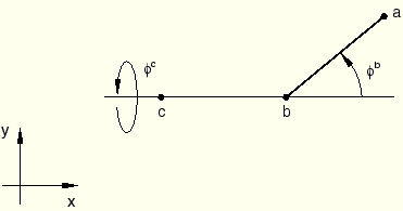
Next, a more rigorous treatment of the two-dimensional constant velocity joint described in “MPC,” Section 25.2.13 of the ABAQUS Analysis User's Manual, is presented. This derivation exemplifies some of the issues associated with the treatment of finite rotations. “Uniform collapse of straight and curved pipe segments,” Section 1.1.5 of the ABAQUS Benchmarks Manual, deals with a different finite rotation constraint and tackles additional complications.
Let ![]() ,
, ![]() ,
, ![]() (see Figure 1.3.1–1) be the nodes making up the joint, with
(see Figure 1.3.1–1) be the nodes making up the joint, with ![]() the dependent node.
the dependent node.
![]()
![]()
![]()
![]()
The linearized constraint is used for the calculation of equilibrium. It can also be used for the recovery of the dependent rotation, ![]() , as is done in the ABAQUS Analysis User's Manual. The resulting rotation will satisfy the constraint approximately (unless one of the angles
, as is done in the ABAQUS Analysis User's Manual. The resulting rotation will satisfy the constraint approximately (unless one of the angles ![]() or
or ![]() is constant, in which case the constraint is linear and the recovery is exact).
is constant, in which case the constraint is linear and the recovery is exact).
For an exact enforcement of the constraint, user subroutine MPC must define the components of the total rotation vector ![]() exactly. To do so,
exactly. To do so, ![]() must be updated based on the current values of
must be updated based on the current values of ![]() and
and ![]() . This is most easily accomplished with the aid of the quaternion parameters. Let
. This is most easily accomplished with the aid of the quaternion parameters. Let ![]() and
and ![]() be the quaternion parameterizations associated with the finite rotation vectors
be the quaternion parameterizations associated with the finite rotation vectors ![]() and
and ![]() , respectively. The total compound rotation
, respectively. The total compound rotation ![]() is given by the quaternion
is given by the quaternion ![]() , where
, where
![]()
![]()
“MPC,” Section 25.2.13 of the ABAQUS Analysis User's Manual, shows the implementation of the linearized form of the constraint in user subroutine MPC. The implementation of the exact nonlinear constraint is shown below:
SUBROUTINE MPC(UE,A,JDOF,MDOF,N,JTYPE,X,U,UINIT,MAXDOF,LMPC,
      * KSTEP,KINC,TIME,NT,NF,TEMP,FIELD)
 C
       INCLUDE 'ABA_PARAM.INC'
 C
       DIMENSION UE(MDOF), A(MDOF,MDOF,N), JDOF(MDOF,N), X(6,N),
      * U(MAXDOF,N), UINIT(MAXDOF,N), TIME(2), TEMP(NT,N),
      * FIELD(NF,NT,N)
       PARAMETER( SMALL = 1.E-14 )
 C
       IF ( JTYPE .EQ. 1 ) THEN
         A(1,1,1) =  1.
         A(2,2,1) =  1.
         A(3,3,1) =  1.
         A(3,1,2) = -1.
         A(1,1,3) = -COS(U(6,2))
         A(2,1,3) = -SIN(U(6,2))
 C
         JDOF(1,1) = 4
         JDOF(2,1) = 5
         JDOF(3,1) = 6
         JDOF(1,2) = 6
         JDOF(1,3) = 4
 C
         CPHIB = COS(0.5*U(6,2))
         SPHIB = SIN(0.5*U(6,2))
         CPHIC = COS(0.5*U(4,3))
         SPHIC = SIN(0.5*U(4,3))
 C
         QA0 = CPHIB*CPHIC
         QAX = CPHIB*SPHIC
         QAY = SPHIB*SPHIC
         QAZ = CPHIB*SPHIC
 C
         QAMAG = SQRT( QAX*QAX + QAY*QAY + QAZ*QAZ )
         IF ( QAMAG .GT. SMALL ) THEN
           PHIA  = 2.*ATAN2( QAMAG , QA0 )
           UE(1) = PHIA*QAX/QAMAG
           UE(2) = PHIA*QAY/QAMAG
           UE(3) = PHIA*QAZ/QAMAG
         ELSE
           UE(1) = 0.
           UE(2) = 0.
           UE(3) = 0.
         END IF
       END IF
 C
       RETURN
       END