Products: ABAQUS/Standard ABAQUS/Explicit
The contact modeling capabilities in ABAQUS allow access to a library of “surface constitutive models.” Part of this library in ABAQUS/Standard is the definition of the contact pressure between two surfaces at a point, ![]() , as a function of the “overclosure,”
, as a function of the “overclosure,” ![]() , of the surfaces (the interpenetration of the surfaces). Two models for
, of the surfaces (the interpenetration of the surfaces). Two models for ![]() are provided as described below.
are provided as described below.
In this case
![]()
The contact constraint is enforced with a Lagrange multiplier representing the contact pressure in a mixed formulation. The virtual work contribution is
![]()
![]()
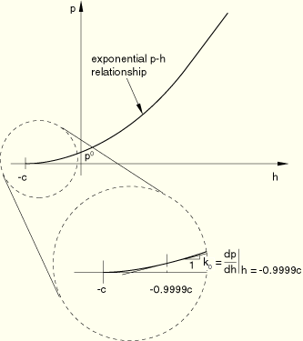
This model provides an exponential ![]() –
–![]() relationship, as shown in Figure 5.2.1–1.
relationship, as shown in Figure 5.2.1–1.
The user defines an initial contact distance, ![]() , and a typical pressure value,
, and a typical pressure value, ![]() , which is the pressure value at zero overclosure (
, which is the pressure value at zero overclosure (![]() ). Then, we define
). Then, we define
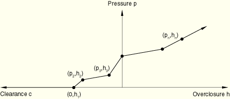
The pressure-overclosure (![]() -
-![]() ) relationship can be entered directly in tabular form as shown in Figure 5.2.1–2.
) relationship can be entered directly in tabular form as shown in Figure 5.2.1–2.
The linear pressure-overclosure relationship is similar to the tabular relationship except that the linear form requires only a single value to be input to define the slope and the curve always passes through the origin.
A mixed formulation is used because the exponential stiffness associated with softened contact tends to slow down convergence or, due to the development of excessive contact stresses, may cause divergence. For the mixed formulation the virtual work contribution is
where![]()
![]()
Substituting for the pressure ![]() in Equation 5.2.1–1 and Equation 5.2.1–2, we obtain
in Equation 5.2.1–1 and Equation 5.2.1–2, we obtain
![]()
![]()
In the mixed formulation the difference between the actual and the calculated overclosure ![]() will go to zero as part of the iterative solution process. The difference must be sufficiently small to obtain an accurate solution. The admissible error in
will go to zero as part of the iterative solution process. The difference must be sufficiently small to obtain an accurate solution. The admissible error in ![]() is set to
is set to ![]() for
for ![]() . For
. For ![]() the admissible error is interpolated linearly between
the admissible error is interpolated linearly between ![]() and
and ![]() , where
, where ![]() represents the tolerance level at
represents the tolerance level at ![]() ; alternatively, the tolerances can be specified by the user as part of the solution controls.
; alternatively, the tolerances can be specified by the user as part of the solution controls.
In addition to the surface constitutive models described above, where the contact pressure is a function of the surface overclosure, ABAQUS/Standard allows for the definition of a “viscous” pressure that is proportional to the relative velocity, ![]() , at which the surfaces approach or separate from each other. This option is intended for the regularization of snap-through problems involving contact where convergence difficulties arise due to the sudden violation of contact constraints.
, at which the surfaces approach or separate from each other. This option is intended for the regularization of snap-through problems involving contact where convergence difficulties arise due to the sudden violation of contact constraints.
The damping pressure, ![]() , is given by
, is given by
![]()
The virtual work contribution associated with the damping pressure is
![]()
In static analysis the velocity is defined as the displacement increment divided by the time increment. Therefore, ![]() , and the stiffness contribution reduces to
, and the stiffness contribution reduces to
![]()
In the case of dynamics ![]() is defined by the dynamic time integration operator, and the stiffness contribution can be written as
is defined by the dynamic time integration operator, and the stiffness contribution can be written as
![]()