In the elastic stick formulation in ABAQUS/Standard, the “elastic” tangential slip is defined as the reversible relative tangential motion from the point of zero shear stress. The elastic slip is related to the interface shear stress with the relation

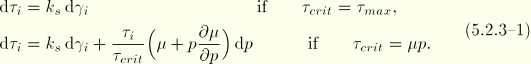
where is the (current) “stiffness in stick,” which follows from the relation Since may be dependent on contact pressure, slip rate, average surface temperature at the contact point, and field variables, may change during the analysis. The behavior remains elastic as long as the equivalent stress does not exceed the critical stress; hence, Consistent linearization of this expression yields The contributions from the contact pressure are nonsymmetric for the second case. Since the slip rate is zero in the elastic stick formulation, derivatives with respect to the slip velocity are not needed.

The above expressions hold if the equivalent shear stress remains less than the critical stress. If the equivalent stress exceeds the critical stress, slip must be taken into consideration so that the condition is satisfied. Let the starting situation be characterized by the elastic slip . The critical stress at the end of the increment follows from the contact pressure, , and the slip rate, .

Let the (as yet unknown) elastic slip at the end of the increment be and the slip increment be . Consistency requires that

and the shear stress at the end of the increment follows from the elasticity relation, The slip increment is related to the stress at the end of the increment with the backward difference approach: With these equations and the critical stress equality it is possible to solve for , , and . Elimination of and from the above equations yields, or It is convenient to define the “elastic predictor strain” which simplifies the expression for the stress to Substitution in the critical stress equality yields where Substitution in the expression for and introduction of the normalized slip direction furnishes the final result Here is a function of the slip rate, which is obtained with where is the time increment in a static analysis. In the case of dynamics is scaled by the Hilber-Hughes-Taylor time integration operator parameters, and .

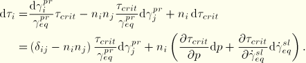
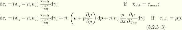
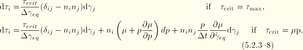
For the iterative solution scheme this equation must be linearized. Some straightforward algebra yields

With the expression for the equivalent slip the final result is In this case the unsymmetric terms may have a strong effect on the speed of convergence of the Newton scheme. Hence, use of the unsymmetric equations solver is strongly recommended for the analysis of problems in which sliding friction occurs. In the case of dynamics is scaled by the Hilber-Hughes-Taylor time integration operator parameters.

If the user specifies different velocities for two bodies in contact as a predefined field, it is assumed that the slip velocity follows from the prescribed motion and is independent of the displacement values. The frictional stresses then follow from

where and are the tangential slip velocities derived from the user-defined fields ().

At the contact nodes at which the velocity differential is imposed, the linearized shear stress can be expressed in the following form:

In the equation above the first term is generated by the friction forces acting in the direction perpendicular to the direction of slip. The third term exists if the friction coefficient depends on velocity. In the complex eigenvalue extraction analysis both terms contribute to the damping matrix. The second term contributes to the stiffness matrix.

For steady-state transport a viscous stick formulation is used. In this case the “viscous” tangential slip rate, , is related to the interface shear stress by

where is the “stick viscosity,” which follows from the relation The allowable viscous slip is defined as a fraction of the relative tangential velocity where is a user-defined slip tolerance, is the angular spinning velocity, and is the radius of a point on the contact surface in the undeformed configuration.

In ABAQUS/Standard Lagrange multipliers are used to enforce exact sticking conditions. A constraint term enforced with Lagrange multipliers is added to the virtual work statement:

where is a Lagrange multiplier. By taking the rate of change of Equation 5.2.3–4, the rate of virtual work is obtained: where the last term results from a nonlinear relation between nodal displacements and relative motion . This term is nonzero only for contact with finite sliding (see “Finite-sliding interaction between deformable bodies,” Section 5.1.2, and “Finite-sliding interaction between a deformable and a rigid body,” Section 5.1.3).

To obtain a complete formulation, a relationship between , , and must be defined. For sticking conditions a suitable relation is

with a reference stiffness selected internally in ABAQUS. The reference stiffness can be considered to model a spring that is in parallel to the sticking constraint. Since the constraint prevents relative motion, the reference stiffness has no physical significance and is added only to eliminate zero terms on the diagonal of the stiffness matrix that could cause equation solver problems. The variational and rate forms of the equation for are readily obtained as Substitution in Equation 5.2.3–5 yields

If the element is slipping, can take an arbitrary value. Consequently the terms involving in Equation 5.2.3–4 and Equation 5.2.3–5 vanish. With the backward difference method, the frictional stress is obtained as

and the linearized form is The rate of virtual work can, hence, be written in the form Observe that for two-dimensional problems the term involving vanishes. In the case of dynamics is scaled by the Hilber-Hughes-Taylor time integration operator parameters.

To determine whether an element sticks or slips, the following tests are used. If the element is currently sticking, it is checked whether the magnitude of the frictional stress exceeds the critical value. Hence, if

the state is changed to slipping.

If the element is slipping, the direction of slip is compared with the frictional stress applied at the start of the iteration. If at the end of the iteration

the state is changed to sticking.

In anisotropic friction the friction coefficients in the two (principal) directions are different; hence, the critical shear stresses are different:

The two critical shear stresses are at the extreme points of the friction ellipse, given by the equation This suggests definition of the scaled shear stresses, where is the average friction coefficient defined by Hence, the (scaled) equivalent frictional stress is defined by and the average critical stress where is the user-specified limiting shear stress, which is applied to the scaled shear stresses. No slip will occur if , and slip can occur if .

If slip occurs, it is assumed that the direction of slip is governed by an associated slip law:

Hence, scaled rates of slip are defined by and the (scaled) equivalent slip rate As a result, the direction of the scaled slip and the scaled shear stress coincide: Since these equations have exactly the same structure as the equations for isotropic friction, the same solution algorithms can be used to get the incremental and linearized equations in terms of the scaled stress and slip. The actual stresses are readily obtained from the scaled stresses with Equation 5.2.3–10, and the linearized equations are scaled with the same factors.

In the anisotropic elastic stick formulation, it is assumed that the stiffness in stick in terms of the scaled stress and slip is constant:

hence, the scaled stress is related to the scaled elastic slip by the relation

In terms of the actual stress and strain in the - and -directions, this implies

with Hence, the anisotropy in terms of the stiffness in stick is more pronounced than the anisotropy in terms of critical stress.

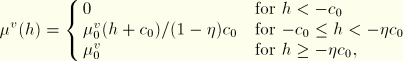
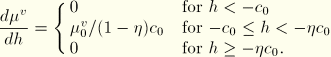
In addition to the friction models described above, ABAQUS allows for the definition of a “viscous” shear stress that is proportional to the relative tangential velocity . This viscous damping in the tangential direction occurs if

The viscous damping stress is proportional to the tangential damping coefficient , which is a function of the overclosure as follows:where is the value of the tangential damping coefficient at zero overclosure and is the fraction of the overclosure interval over which the damping coefficient is equal to .

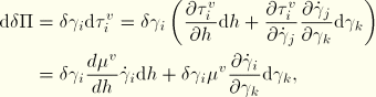
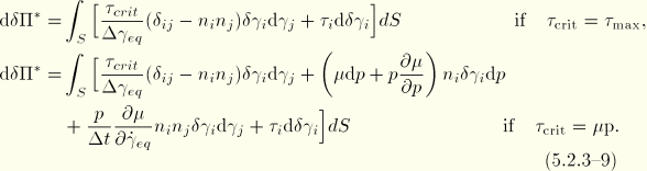
The virtual work contribution associated with the viscous shear stress is

The contribution to the stiffness matrix for the Newton solution is given by the linearized form of the virtual work contribution: where

In static analysis the velocity is defined as the displacement increment divided by the time increment. Therefore, , and the stiffness contribution reduces to

In the case of dynamics is defined by the dynamic time integration operator and the stiffness contribution can be written as

where and are the Hilber-Hughes-Taylor time integration operator parameters. Viscous damping cannot be used in a Riks analysis since velocity is not defined.