Product: ABAQUS/Aqua
An ABAQUS/Aqua analysis:
is used to apply steady current, wave, and wind loading to submerged or partially submerged structures in problems such as the modeling of offshore piping installations or the analysis of marine risers;
can be performed using the static (“Static stress analysis,” Section 6.2.2), direct-integration dynamic (“Implicit dynamic analysis using direct integration,” Section 6.3.2), or eigenfrequency extraction (“Natural frequency extraction,” Section 6.3.5) procedures;
will calculate drag, buoyancy, and inertia loading only for beam, pipe, elbow, truss, and certain rigid elements;
can include elements that model spud cans for jack-up foundation analysis; and
can be linear or nonlinear.
Aqua loading can be applied in static steps (“Static stress analysis,” Section 6.2.2) and in direct-integration dynamic steps (“Implicit dynamic analysis using direct integration,” Section 6.3.2). During these steps fluid particle velocity is assumed to consist of two superposed effects: steady currents, which can vary with elevation and location, and gravity waves. Fluid particle accelerations are associated with gravity waves only.
The fluid particle velocities and accelerations are used to calculate drag and inertia loading on the immersed body. ABAQUS/Aqua also computes the fluid surface elevation and allows for partial immersion; drag and buoyancy loadings are omitted for those parts of the structure that are above the fluid surface or below the seabed level.
An eigenfrequency extraction step (“Natural frequency extraction,” Section 6.3.5) can be used to extract the natural frequencies of a structure prestressed by the Aqua loading in a static or direct-integration dynamic step (if that step included the effects of nonlinear geometry). The added-mass effect due to fluid inertia loads can be included in an eigenfrequency extraction step.
Aqua loads are applied in the following manner:
The fluid properties and steady current velocity are defined for the model.
Gravity waves and wind velocity are defined for the model.
Drag, buoyancy, and fluid inertia loads are applied to elements and nodes of the structure using distributed or concentrated load definitions within the static or direct-integration dynamic step definition. The magnitudes of the loads applied are determined by the fluid properties, steady current, wave, and wind definitions.
In an eigenfrequency extraction step concentrated and distributed added mass definitions are used (instead of concentrated and distributed loads) to include the effects of fluid inertia.
On the other hand, if a relatively stiff structure is subject to Aqua loads or if a dynamic step uses small time increments, the unsymmetric load-stiffness terms may not be dominant and you may be able to obtain a convergent solution with the symmetric solver (see, for example, “Riser dynamics,” Section 10.1.2 of the ABAQUS Example Problems Manual).
The z-coordinate axis must point vertically for three-dimensional cases, and the y-coordinate axis must point vertically for two-dimensional cases. For the three-dimensional case the still fluid surface (when there is no wave motion) lies in a plane that is parallel to the x–y plane. For the two-dimensional case it lies parallel to the x-axis. The position of the still fluid surface is specified as part of the fluid property data.
Aqua loadings require the definition of fluid density, seabed and free surface elevation, and the gravitational constant.
Steady currents are defined by giving steady fluid velocity as a function of elevation and location. Elevation is defined in the positive z-direction for three-dimensional models and in the positive y-direction for two-dimensional models. For two-dimensional cases the z-component of the steady current velocity is ignored. See “Input syntax rules,” Section 1.2.1, for an explanation of how to define one property (in this case steady current velocity) as a function of multiple independent variables.
If the fluid velocity is not a function of elevation or location (for example, when modeling a problem in a coordinate system that moves uniformly through the still fluid, such as a tow-out analysis), only one fluid velocity need be specified.
The steady current velocities can be scaled by referring to an amplitude curve (“Amplitude curves,” Section 27.1.2) from the concentrated or distributed load definitions used to apply drag loads, as described later.
| Input File Usage: | *AQUA fluid properties on first data line (described above) X-velocityfluid, Y-velocityfluid, Z-velocityfluid, elevation, X-coord, Y-coord ... |
You can define gravity waves. The fluid velocity and acceleration due to the gravity waves are used to apply drag and buoyancy loadings.
You can choose Airy linear wave theory, Stokes fifth-order wave theory, wave data read from a gridded mesh, or fluid kinematics defined in user subroutine UWAVE. For Airy and Stokes waves the fluid surface elevation and the fluid particle velocities and accelerations will be calculated as functions of time and location based on the wave definition. If wave data are provided in the form of a gridded mesh, you must specify these quantities. If user subroutine UWAVE is used, the fluid kinematics must be defined in that routine.
All of the built-in wave theories assume a series of waves in the horizontal plane (the plane of the fluid surface) that are unaffected by any fluid-structural interaction. The Airy and Stokes theories are based on irrotational flow of an inviscid, incompressible fluid, where the wave height H is small compared to the still water depth d. The bottom of the fluid is assumed to be flat (the still water depth is constant).
The Ursell parameter,
![]()
Linear Airy wave theory is generally used when the ratio of wave height to water depth, ![]() , is less than 0.03, provided that the water is deep (ratio of water depth to wavelength,
, is less than 0.03, provided that the water is deep (ratio of water depth to wavelength, ![]() , is greater than 20). Convective acceleration terms are neglected in the Airy theory as part of the linearization. The Airy wave theory is described in detail in “Airy wave theory,” Section 6.2.2 of the ABAQUS Theory Manual.
, is greater than 20). Convective acceleration terms are neglected in the Airy theory as part of the linearization. The Airy wave theory is described in detail in “Airy wave theory,” Section 6.2.2 of the ABAQUS Theory Manual.
Since the Airy wave theory is linear, any number of wave trains traveling in different directions across the water can be defined; the fluid particle velocities and accelerations sum by linear superposition. The direction of each wave component is given by specifying the direction cosines of a vector, ![]() , lying in the plane defined by the still fluid surface.
, lying in the plane defined by the still fluid surface.
By default, Airy waves are defined in terms of wavelength, ![]() . Alternatively, you can define the waves in terms of wave period,
. Alternatively, you can define the waves in terms of wave period, ![]() . For Airy wave theory the wavelength and period of each component are related by
. For Airy wave theory the wavelength and period of each component are related by
![]()
![]()
is the period of this component,
g
is the gravitational acceleration,
![]()
is the wavelength, and
h
is the undisturbed (still) water depth.
| Input File Usage: | Use the following option to define an Airy wave in terms of wavelength: |
*WAVE, TYPE=AIRY
amplitude, wavelength, phase angle, x-direction cosine, y-direction cosine
Use the following option to define an Airy wave in terms of wave period: *WAVE, TYPE=AIRY, WAVE PERIOD amplitude, wave period, phase angle, x-direction cosine, y-direction cosine In either case repeat the data line to define multiple wave trains. |
The Stokes fifth-order wave theory is a deep-water wave theory that is valid for relatively large wavelengths. Convective terms are included in the fluid particle acceleration calculations for Stokes fifth-order theory and can be significant for larger ![]() ratios. The Stokes wave theory is described in detail in “Stokes wave theory,” Section 6.2.3 of the ABAQUS Theory Manual.
ratios. The Stokes wave theory is described in detail in “Stokes wave theory,” Section 6.2.3 of the ABAQUS Theory Manual.
Because the Stokes fifth-order wave theory is nonlinear, only one wave train is allowed in an analysis. The relationship between wavelength and period of the waves in Stokes fifth-order theory is not as simple as that for the Airy theory, although the formula given above is a first-order approximation. Stokes waves can be defined only in terms of the wave period, ![]() .
.
| Input File Usage: | *WAVE, TYPE=STOKES wave height, wave period, phase angle, direction of travel cosines |
You can choose to provide wave surface elevations, particle velocities and accelerations, and the dynamic pressure at points in a user-defined grid through a binary data file. The binary file contains information about the wave definition, the location of the grid points where wave information is specified, and the wave kinematics at user-defined times. At spatial locations within the user-defined grid, ABAQUS/Aqua will interpolate the wave kinematics from the nearest grid points, using either linear or quadratic interpolation. When a point on the structure is above the user-defined grid, ABAQUS/Aqua assumes that the point is above the free surface elevation. Hence, no fluid loads are applied. If a point on the structure falls outside the user-defined spatial grid without being above the grid, ABAQUS/Aqua finds the wave kinematics at the nearest point within the grid and uses those values at the point on the structure.
| Input File Usage: | *WAVE, TYPE=GRIDDED, DATA FILE=file_name |
The data file must contain the following unformatted (binary) records (see “Aqua load cases,” Section 3.10.1 of the ABAQUS Verification Manual). The data for the FORTRAN WRITE statement are given for each record:
First record:
NCOMP, DTG, NWGX, NWGY, NWGZ, IPDYNwhere
NCOMP
is the number of wave components to be read in the data file;
DTG
is the time increment at which wave data are given on the grid;
NWGX
is the number of grid points in the grid's x-direction;
NWGY
is the number of grid points in the grid's y-direction—if this number is one, ABAQUS/Aqua assumes that the wave data are constant with respect to the local y-direction;
NWGZ
is the number of grid points in the grid's z-direction—if this number is zero or one, the analysis is two-dimensional and the y-direction is vertical; and
IPDYN
is an integer flag indicating whether dynamic pressure information is stored (IPDYN=1) or not stored (IPDYN=0) in the gridded wave file.
Second record:
(AMP(K1), WXL(K1), PHI(K1), K1=1,NCOMP)where
NCOMP
is read on the first record, above;
AMP
contains the wave component amplitude, ![]() ;
;
WXL
contains the wavelength of this component, ![]() ; and
; and
PHI
contains the phase angle of this component, ![]() (in degrees).
(in degrees).
Third record:
(WGX(K1),K1=1,NWGX), (WGY(K1),K1=1,NWGY), (WGZ(K1),K1=1,NWGZ)where
NWGi
are read on the first record, above;
WGX
contains the local x-coordinates of the grid points;
WGY
contains the local y-coordinates of the grid points; and
WGZ
contains the local z-coordinates of the grid points (not included in the gridded wave file for two-dimensional analyses).
For three dimensions:
(((WGVX(K1,K2,K3), WGVY(K1,K2,K3), WGVZ(K1,K2,K3),
WGAX(K1,K2,K3), WGAY(K1,K2,K3), WGAZ(K1,K2,K3), K3=1,NWGZ),
WZCRST(K1,K2), NCRST(K1,K2), K1=1,NWGX), K2=1,NWGY)
For two dimensions:
((WGVX(K1,K2), WGVY(K1,K2), WGAX(K1,K2), WGAY(K1,K2),
K2=1,NWGY), WZCRST(K1), NCRST(K1), K1=1,NWGX)
Remaining records if IPDYN=1:
For three dimensions:
(((WGVX(K1,K2,K3), WGVY(K1,K2,K3), WGVZ(K1,K2,K3),
WGAX(K1,K2,K3), WGAY(K1,K2,K3), WGAZ(K1,K2,K3),
P(K1,K2,K3), DPDZ(K1,K2,K3), K3=1,NWGZ),
WZCRST(K1,K2), NCRST(K1,K2), K1=1,NWGX), K2=1,NWGY)
For two dimensions:
((WGVX(K1,K2), WGVY(K1,K2), WGAX(K1,K2), WGAY(K1,K2),
P(K1,K2), DPDZ(K1,K2), K2=1,NWGY),
WZCRST(K1), NCRST(K1), K1=1,NWGX)
where
WGVX
contains the local x-components of the wave particle velocity,
WGVY
contains the local y-components of the wave particle velocity,
WGVZ
contains the local z-components of the wave particle velocity,
WGAX
contains the local x-components of the wave particle acceleration,
WGAY
contains the local y-components of the wave particle acceleration,
WGAZ
contains the local z-components of the wave particle acceleration,
WZCRST
contains the wave surface elevation,
NCRST
contains the index for the vertical grid level just above the instantaneous water surface,
P
contains the dynamic pressure, and
DPDZ
contains the gradient of the dynamic pressure in the vertical direction.
A user-defined wave theory can be coded in user subroutine UWAVE. The user subroutine must define the fluid particle velocity and acceleration, free surface elevation, and dynamic pressure field.
| Input File Usage: | *WAVE, TYPE=USER |
For stochastic analysis you can specify a random number seed, r, and define frequency/amplitude pairs that define the wave spectrum. During the analysis ABAQUS/Aqua stores an intermediate configuration that can be used in the user subroutine to compute the stochastic description of the waves. The intermediate configuration is initialized as the reference configuration and is replaced by the current configuration only when requested by the user subroutine. In this way the stochastic description of the wave field can be stored in an external database and recalculated only when necessary.
| Input File Usage: | *WAVE, TYPE=USER, STOCHASTIC=r frequency, amplitude ... |
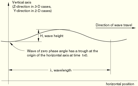
For Airy and Stokes waves the position of the wave at time ![]() can be chosen by specifying the phase angle
can be chosen by specifying the phase angle ![]() of the wave (or wave components for Airy waves). By default, the waves are chosen such that they have a trough (vertical displacement of the fluid surface is a minimum) at the origin of the horizontal axes at time
of the wave (or wave components for Airy waves). By default, the waves are chosen such that they have a trough (vertical displacement of the fluid surface is a minimum) at the origin of the horizontal axes at time ![]() . You can change this trough by introducing a phase angle
. You can change this trough by introducing a phase angle ![]() for the waves. A positive phase angle shifts the waves backward in their travel direction (see Figure 6.10.1–1).
for the waves. A positive phase angle shifts the waves backward in their travel direction (see Figure 6.10.1–1).
The time t used in the wave theory is the total time in the analysis. Therefore, if the direct-integration dynamic steps in which Airy or Stokes waves are applied are preceded by any steps other than direct-integration dynamic steps (such as static steps), it is usually convenient to make the time period in these steps very small compared to the period of the wave.
Because total time is used, the phase of the wave will be continuous from the end of one dynamic step to the beginning of the next dynamic step.
For computational efficiency ABAQUS/Aqua uses a minimum wave trough elevation below which the structure is assumed to be immersed. Below this elevation no calculation of the fluid surface need be done to determine if the point of interest is above the instantaneous free surface. Similarly, a maximum wave elevation is used: any point above the maximum wave elevation is assumed to have no fluid loading.
For Airy and Stokes waves the minimum and maximum wave elevations are calculated from the wave theory.
For gridded waves ABAQUS/Aqua allows the definition of a minimum wave trough elevation: ![]() in three-dimensional analysis or
in three-dimensional analysis or ![]() in two-dimensional analysis. The structure is always assumed to be immersed below this elevation. The maximum wave elevation is calculated as the still water elevation plus the difference between this elevation and the minimum wave trough elevation. If the minimum wave trough elevation is not specified for gridded waves, ABAQUS/Aqua will compare the elevation of every point on the structure with the instantaneous fluid surface as defined by the gridded data. When defining this elevation, make sure that no wave trough ever drops below the minimum wave trough elevation specified.
in two-dimensional analysis. The structure is always assumed to be immersed below this elevation. The maximum wave elevation is calculated as the still water elevation plus the difference between this elevation and the minimum wave trough elevation. If the minimum wave trough elevation is not specified for gridded waves, ABAQUS/Aqua will compare the elevation of every point on the structure with the instantaneous fluid surface as defined by the gridded data. When defining this elevation, make sure that no wave trough ever drops below the minimum wave trough elevation specified.
| Input File Usage: | *WAVE, TYPE=GRIDDED, DATA FILE=file_name, MINIMUM=elevation |
A spatial (Eulerian) description of the wave field is used for all wave types; therefore, a structural point's coordinates are used to evaluate the wave kinematics. In geometrically nonlinear analysis the structural point's coordinates are its current coordinates. In geometrically linear analysis the wave kinematics are evaluated using the structural point's reference coordinates.
In both geometrically linear and nonlinear analysis for both static and direct-integration dynamic procedures, submergence is calculated to the instantaneous water level at the current value of total time for the analysis. Fluid loading is applied only to those points on the structure below the instantaneous water level.
When buoyancy loading is applied in conjunction with a gravity wave, the dynamic pressure due to the disturbance of the still surface is added to the hydrostatic pressure (measured to the still water level) to obtain the total buoyancy loading, except when the buoyancy loading described by a distributed or concentrated load definition overrides the fluid properties given for the ABAQUS/Aqua analysis. Dynamic pressure is included for both static and dynamic procedures for Airy, Stokes, and gridded wave types; however, with gridded wave data you can choose to suppress this effect. See “Airy wave theory,” Section 6.2.2 of the ABAQUS Theory Manual, and “Stokes wave theory,” Section 6.2.3 of the ABAQUS Theory Manual, for a definition of dynamic pressure.
Although the linearized Airy wave theory assumes that the fluid displacements are small with respect to the wavelength and the fluid depth, these displacements may not be small with respect to the dimensions of the structure immersed in the fluid. As a result of the linearizing approximations special treatment is necessary to calculate the wave kinematics for points below the instantaneous water level but above the still water line. ABAQUS/Aqua uses extrapolation with Airy wave theory: the wave velocity, acceleration, and dynamic pressure for points above the still water level but below the instantaneous free surface are taken to be the values evaluated from the wave theory at the still water level. See “Airy wave theory,” Section 6.2.2 of the ABAQUS Theory Manual, for more details.
The data for the gravity wave can be contained in an alternate file. See “Input syntax rules,” Section 1.2.1, for the syntax of the file name.
| Input File Usage: | *WAVE, INPUT=file_name |
You can define a wind velocity profile. Wind loading is applied only to elements above the still water surface elevation (defined in the fluid properties). If an element is above the still water depth but is submerged due to a wave, the wind loading will still be applied.
The wind profile is assumed to vary with height (the positive z-direction in three-dimensional models, the positive y-direction in two-dimensional models) according to the power law wind profile and has no variation in the horizontal plane. The power law wind velocity profile is given by
![]()
![]()
![]() is the local wind velocity (
is the local wind velocity (![]() is a unit vector along the local x-axis of the wind field, and
is a unit vector along the local x-axis of the wind field, and ![]() is a unit vector along the local y-axis of the wind field);
is a unit vector along the local y-axis of the wind field);
![]()
is the time-varying wind velocity at the reference height, ![]() , as described below;
, as described below;
![]()
is a user-defined constant (default value 1/7);
z
is the distance above the still water surface (i.e., ![]() is the still water surface); and
is the still water surface); and
![]()
is the reference distance above the still water surface where the time variation of the wind velocity is given.
The wind local system is defined by giving the direction cosines of the unit vector ![]() .
.
| Input File Usage: | *WIND air density, |
The variation in time of the wind profile is defined by ![]() , the wind velocity vector time history at a reference height
, the wind velocity vector time history at a reference height ![]() :
:
![]()
![]()
In geometrically linear analysis wind velocities are calculated based on the original coordinates of the structure. In geometrically nonlinear analysis the current coordinates of a point on the structure are used to calculate the wind velocity at that point.
Initial conditions can be applied to the structure in an ABAQUS/Aqua analysis in the same way as in static and dynamic analyses without Aqua loads. See “Initial conditions,” Section 27.2.1.
Boundary conditions can be applied to the structure in an ABAQUS/Aqua analysis in the same way as in static and dynamic analyses without Aqua loads. See “Boundary conditions,” Section 27.3.1.
Aqua loads are applied only above the seabed. To model the bottom of the sea using a contact plane, the elevation of the contact plane must be slightly higher than the seabed level to avoid ambiguity between the contact condition and applied loading. If the contact plane is at the same level as the seabed, there is a risk that round-off problems will cause Aqua loads not to be applied to nodes in contact with the seabed.
Steady current, wave, and wind loads are applied to nodes or elements of the structure using concentrated and/or distributed load definitions. Wind loads are applied only if the point is currently above the still fluid surface; fluid loads are applied only if the point is currently below the instantaneous fluid surface and above the seabed.
Concentrated and distributed load definitions cannot be used in eigenfrequency extraction steps, so the loads described below can be applied only in static and direct-integration dynamic steps.
You have three ways to control the magnitude of an Aqua load as a function of time:
You can reference a user-defined amplitude curve (“Amplitude curves,” Section 27.1.2) from the concentrated or distributed load definition to scale the entire load.
You can specify a magnitude factor, M, for the concentrated or distributed load definition, which is used to scale all the load. This magnitude factor allows normalized amplitude curves to be defined and used for multiple loads. The default magnitude factor is always ![]() .
.
You can reference individual user-defined amplitude curves to scale different components of the loading separately. For example, steady current velocity and wave velocity can be scaled separately by referencing different amplitude curves.
The calculated buoyancy of a structure depends on the orientation of the exposed surface area with respect to the vertical direction. This surface area is calculated automatically by ABAQUS/Aqua for distributed buoyancy loading; however, you must specify the exposed area and direction cosines of the outward normal at a node for concentrated buoyancy loading.
ABAQUS/Aqua uses a closed-end loading condition while computing the distributed buoyancy forces on all line elements. To obtain an open-end loading condition, concentrated buoyancy loading can be used to counteract the buoyancy load applied to the ends of the elements.
The buoyancy loads require the definition of fluid density, seabed and free surface elevation, and the gravitational constant. The default external fluid properties are defined for the model as described in “Defining the fluid properties.” You can override some of these properties by specifying them directly in the distributed or concentrated load definition. This provides for modeling situations where different parts of the structure are subjected to different buoyancy loads, such as a pipe inside another pipe where the fluid surrounding one pipe is different from that of the other.
To apply distributed buoyancy loads to elements immersed in a fluid, the effective outer diameter of beam, truss, and one-dimensional rigid elements must be specified. Provide the external fluid density, free surface elevation, and additional pressure to override the default fluid properties. For situations where it is necessary to model the fluid inside an element, the effective inner diameter of the element must also be given, along with the density and free surface elevation of the fluid inside the element.
Distributed buoyancy loading can be applied to rigid surface elements. However, the effects of waves are ignored for these elements; the buoyancy loading is calculated to the still water level only. For proper application of a positive buoyancy force, the positive normal of R3D3 and R3D4 elements must point into the fluid.
| Input File Usage: | *DLOAD element number or set, PB, M, effective outer diameter, internal fluid density, effective inner diameter, internal free surface elevation, external fluid density, external free surface elevation, additional pressure |
For concentrated buoyancy loads applied to nodes immersed in a fluid, the load is calculated based on the sum of the hydrostatic pressure (measured to the still water level) and the dynamic pressure due to wave action. The total pressure is multiplied by the exposed area associated with the node. The loading is automatically considered to be a follower force in geometrically nonlinear analysis (for elements that have rotational degrees of freedom); therefore, it is not necessary to specify that the load is a follower force. Provide the external fluid density, free surface elevation, and additional pressure to override the default fluid properties.
| Input File Usage: | *CLOAD node number or set, TSB, M, exposed area, local coordinate system data, external fluid density, external free surface elevation, additional pressure |
Both waves and wind can cause drag loading on a structure. Fluid drag refers to drag caused by the structural member being immersed in the fluid defined by the fluid properties and the gravity waves and, thus, subject to steady current and wave loading. Fluid drag loading is provided by Morison's equation. Fluid drag loads must be specified in terms of a normal (transverse) load and a tangential load.
Wind drag is generated on the portions of a structure that are above the still fluid surface defined by the fluid properties because these portions are exposed to the user-defined wind velocity profile.
Distributed transverse drag is defined as follows (see “Drag, inertia, and buoyancy loading,” Section 6.2.1 of the ABAQUS Theory Manual, for more details):
![]()
![]()
is the force per unit length, transverse to the member;
![]()
is the current value of the amplitude curve referred to by the distributed load definition, multiplied by the user-defined magnitude factor, M;
![]()
is the mass density of the fluid (given in the fluid properties) for fluid distributed drag or is the mass density of the air (given in the wind velocity profile) for wind distributed drag;
![]()
is the drag coefficient; and
D
is the effective outer diameter of the member.
![]()
![]()
is the fluid particle velocity (see the discussion below);
![]()
is the velocity of this point on the structure (zero during static steps);
![]()
is the structural velocity factor; and
![]()
is the unit vector along the axis of the element.
The velocities due to steady current and waves can be scaled individually for fluid distributed drag by referring to different amplitude curves. Thus, the fluid particle velocity, ![]() , at any time is
, at any time is
![]()
![]()
is the current value of the first amplitude curve listed in the load definition or 1.0 if the amplitude reference is omitted,
![]()
is the steady current velocity defined in the fluid properties,
![]()
is the current value of the second amplitude curve listed in the load definition or 1.0 if the amplitude reference is omitted, and
![]()
is the user-defined wave velocity.
The wind velocity is defined in components relative to the local axes ![]() and
and ![]() defined for the wind velocity profile. Each velocity component can be scaled independently by referring to different amplitude curves. The total wind velocity at any time,
defined for the wind velocity profile. Each velocity component can be scaled independently by referring to different amplitude curves. The total wind velocity at any time, ![]() , is
, is
![]()
Distributed tangential fluid loading is a load in the tangential direction of an element due to skin friction. This type of loading is defined as follows (see “Drag, inertia, and buoyancy loading,” Section 6.2.1 of the ABAQUS Theory Manual, for more details):
![]()
![]()
is the force per unit length, tangent to the member;
![]()
is the amplitude curve referred to by the distributed load definition, multiplied by the user-defined magnitude factor, M;
![]()
is the mass density of the fluid (given in the fluid properties);
![]()
is the tangential drag coefficient;
D
is the effective outer diameter of the member; and
h
is a constant (by default, ![]() , for quadratic dependence of force on velocity).
, for quadratic dependence of force on velocity).
![]()
![]()
is the fluid particle velocity (as defined above for distributed transverse fluid drag loading),
![]()
is the velocity of this point on the structure (zero during static steps),
![]()
is the structural velocity factor, and
![]()
is the unit vector along the axis of the element.
As with distributed transverse fluid loading, the velocities due to steady current and waves (![]() and
and ![]() ) can be scaled individually by referring to different amplitude curves.
) can be scaled individually by referring to different amplitude curves.
| Input File Usage: | Use the following option to define fluid drag tangential: |
*DLOAD element number or set, FDT, M, D, |
Concentrated fluid or wind drag loading applies a load normal to the end of an element. Such loading is automatically considered to be a follower force in geometrically nonlinear analysis (for elements that have rotational degrees of freedom).
The drag theory uses Morison's equation (see “Drag, inertia, and buoyancy loading,” Section 6.2.1 of the ABAQUS Theory Manual). The drag force is nonzero when the net flow is in the opposite direction of the outward normal to the exposed area and is zero when the net flow is in the direction of the normal:
![]()
![]()
is the amplitude curve referenced by the concentrated load definition multiplied by the user-defined magnitude factor, M;
![]()
is the mass density of the fluid (given in the fluid properties) for transition section fluid drag or is the mass density of the air (given in the wind velocity profile) for transition section wind drag;
![]()
is the drag coefficient;
![]()
is the exposed area; and
![]()
is the relative velocity between the structural member and the fluid particle along ![]() and is given by
and is given by ![]() , where
, where ![]() as defined above for distributed tangential fluid drag loading.
as defined above for distributed tangential fluid drag loading.
The exposed area, ![]() ; the drag coefficient,
; the drag coefficient, ![]() ; and the structural velocity factor,
; and the structural velocity factor, ![]() , must be defined in the concentrated load definition together with the concentrated load type (transition section fluid drag or transition section wind drag).
, must be defined in the concentrated load definition together with the concentrated load type (transition section fluid drag or transition section wind drag).
As with distributed transverse fluid loading, the velocities due to steady current and waves (![]() and
and ![]() ) and the velocity components of the wind in the
) and the velocity components of the wind in the ![]() and
and ![]() directions (
directions (![]() and
and ![]() ) can be scaled individually by referring to different amplitude curves.
) can be scaled individually by referring to different amplitude curves.
You can apply concentrated fluid or wind drag loading on the ends of elements. These loads have the same effect as specifying a concentrated load at a node using a concentrated load definition with concentrated load type transition section fluid drag or transition section wind drag, except that the normal to the exposed area cannot be specified when a distributed load definition is used; the normal to the end of the element is defined by the tangent to the element.
The load can be applied to the first end (node) of the element or to the second end (node 2 or 3, as appropriate) of the element. These loads are nonzero only when the net flow is in the opposite direction of the outward normal to the exposed area.
The loading is exactly the same as that described for the concentrated fluid or wind drag loading applied with a concentrated load definition. The “distributed” form of the loading is provided for convenience.
| Input File Usage: | Use the following option to define fluid drag on the first end of the element: |
*DLOAD element number or set, FD1, M, Use the following option to define fluid drag on the second end of the element: *DLOAD element number or set, FD2, M, Use the following option to define wind drag on the first end of the element: *DLOAD element number or set, WD1, M, Use the following option to define wind drag on the second end of the element: *DLOAD element number or set, WD2, M, |
If the wave's contribution to the drag and inertia loading should not be applied during a step, the concentrated or distributed load component definition must explicitly refer to an amplitude curve with a value of zero. This is the only way to prevent waves from contributing to the fluid velocities and accelerations used in the calculation of these concentrated or distributed load types.
Fluid inertia loading causes a structure to have increased inertial resistance to acceleration. This fluid “added-mass” effect is included automatically in a direct-integration dynamic step when fluid inertia loading is applied. Concentrated or distributed added mass must be defined to include the added-mass effect in an eigenfrequency extraction step.
Distributed fluid inertia loading is defined as follows (see “Drag, inertia, and buoyancy loading,” Section 6.2.1 of the ABAQUS Theory Manual, for a more detailed description):
![]()
![]()
is the force per unit length, transverse to the member, caused by fluid inertia;
![]()
is the amplitude curve referred to by the distributed load definition multiplied by the user-defined magnitude factor, M;
![]()
is the mass density of the fluid (given in the fluid properties);
D
is the effective outer diameter of the member;
![]()
is the transverse fluid inertia coefficient;
![]()
is the transverse added-mass coefficient;
![]()
is the transverse component of the fluid acceleration; and
![]()
is the transverse component of the beam acceleration (zero during static steps).
The fluid acceleration, ![]() , is calculated according to the user-defined gravity wave and is further scaled by the amplitude curve,
, is calculated according to the user-defined gravity wave and is further scaled by the amplitude curve, ![]() , referred to by the distributed load definition.
, referred to by the distributed load definition.
| Input File Usage: | Use the following option to define distributed fluid inertia in a dynamic step: |
*DLOAD element number or set, FI, M, D, |
The added mass contribution due to distributed fluid inertia loading is
![]()
![]()
is the mass density of the fluid (given in the fluid properties),
D
is the effective outer diameter of the member, and
![]()
is the transverse added-mass coefficient.
| Input File Usage: | *D ADDED MASS element number or set, FI, D, |
Concentrated fluid inertia loading is automatically considered to be a follower force (for elements that have rotational degrees of freedom).
The inertia term is calculated as a force in the current direction of the outward normal to the exposed surface area:
![]()
![]()
is the point force caused by fluid inertia;
![]()
is the amplitude curve referenced by the concentrated load definition multiplied by the user-defined magnitude factor, M;
![]()
is the mass density of the fluid (given in the fluid properties);
![]()
is the tangential inertia coefficient;
![]()
is the fluid acceleration shape factor (of dimension ![]() );
);
![]()
is the tangential added-mass coefficient;
![]()
is the structural acceleration shape factor (of dimension ![]() );
);
![]()
is the fluid acceleration in the direction of the outward normal to the exposed surface; and
![]()
is the structural acceleration in the direction of the outward normal to the exposed surface (zero during static steps).
The fluid acceleration, ![]() , is calculated according to the user-defined gravity wave and is further scaled by the amplitude curve,
, is calculated according to the user-defined gravity wave and is further scaled by the amplitude curve, ![]() , referred to by the concentrated load definition.
, referred to by the concentrated load definition.
| Input File Usage: | Use the following option to define transition section inertia in a dynamic step: |
*CLOAD node number or set, TSI, M, |
You can apply concentrated fluid inertia loading at the ends of elements. These loads have the same effect as specifying a concentrated fluid added-inertia loading using a concentrated load definition with concentrated load type transition section inertia, except that the normal to the exposed area cannot be specified when a distributed load definition is used; the normal to the end of the element is defined by the tangent to the element.
The inertia loading can be applied to the first end (node) of the element or to the second end (node 2 or 3, as appropriate) of the element.
The loading is exactly the same as that described for the concentrated fluid inertia loading applied with a concentrated load definition. The “distributed” form of the loading is provided for convenience.
| Input File Usage: | Use the following option to define fluid inertia on the first end of the element in a dynamic step: |
*DLOAD element number or set, FI1, M, Use the following option to define fluid inertia on the second end of the element in a dynamic step: *DLOAD element number or set, FI2, M, |
The added mass contribution due to concentrated fluid inertia loading in an eigenfrequency extraction step is
![]()
![]()
is the mass density of the fluid (given in the fluid properties),
![]()
is the tangential added-mass coefficient, and
![]()
is the structural acceleration shape factor (of dimension ![]() ).
).
| Input File Usage: | *C ADDED MASS node number or set, TSI, |
You can apply concentrated fluid inertia effects at the ends of elements. These loads have the same effect as specifying concentrated fluid inertia effects using a concentrated added mass definition with concentrated load type transition section inertia, but in this case the normal to the exposed area cannot be specified; the normal to the end of the element is defined by the tangent to the element.
The added mass can be applied to the first end (node) of the element or to the second end (node 2 or 3, as appropriate) of the element.
The effect is exactly the same as that described for the concentrated fluid inertia effects applied with a concentrated added mass definition. The “distributed” form of the loading is provided for convenience.
| Input File Usage: | Use the following option to define fluid inertia on the first end of the element in an eigenfrequency extraction step: |
*D ADDED MASS element number or set, FI1, Use the following option to define fluid inertia on the second end of the element in an eigenfrequency extraction step: *D ADDED MASS element number or set, FI2, |
Concentrated and distributed load definitions can also be used to apply concentrated and distributed forces that are not associated with wind, waves, or steady current to the structure. See “Concentrated loads,” Section 27.4.2, and “Distributed loads,” Section 27.4.3.
The following predefined fields can be specified for the structure (not the fluid) in an ABAQUS/Aqua analysis, as described in “Predefined fields,” Section 27.6.1:
Temperatures of nodes in the structure can be specified. Any difference between the applied and initial temperatures will cause thermal strain if a thermal expansion coefficient is given for the material (“Thermal expansion,” Section 20.1.2). The specified temperature also affects temperature-dependent material properties, if any.
The values of user-defined field variables can be specified. These values affect only field-variable-dependent material properties, if any.
Any of the mechanical constitutive models in ABAQUS/Standard can be used for modeling the structure in an ABAQUS/Aqua analysis (see Part V, “Materials,” for details on the material models available in ABAQUS/Standard).
The fluid loads in an ABAQUS/Aqua analysis cannot be applied to all element types: only the beam, pipe, elbow, truss, and rigid beam elements in ABAQUS/Standard can be used to subject a structure to general ABAQUS/Aqua loading. The only load that can be applied to two-dimensional rigid surfaces (R3D3 and R3D4 elements) is hydrostatic buoyancy; current, wave, and wind loading will have no effect.
ABAQUS/Standard provides element types JOINT2D and JOINT3D, which can be used to model elastic-plastic interaction between spud cans and the sea floor (see “Elastic-plastic joints,” Section 26.11.1).
In addition to the usual output variables available in ABAQUS/Standard (see “ABAQUS/Standard output variable identifiers,” Section 4.2.1), element section output variable ESF1 can be used to request output of the effective axial force in a beam subjected to pressure loading (see “Beam element library,” Section 23.3.8). The velocities and accelerations of the fluid cannot be output.
*HEADING
…
*AQUA
Data lines defining the fluid properties and steady current velocity
*WAVE, TYPE=wave theory
Data lines defining gravity waves
**
*STEP (, NLGEOM)
Use the NLGEOM parameter to include nonlinear geometric effects
*DYNAMIC (or *STATIC)
…
*CLOAD
Data lines defining concentrated buoyancy, fluid/wind drag, and fluid inertia loads
*DLOAD
Data lines defining distributed buoyancy, fluid/wind drag, and fluid inertia loads
*END STEP
**
*STEP
The NLGEOM parameter must have been included in the previous step to obtain
the natural frequencies of the prestressed structure
*FREQUENCY
…
*C ADDED MASS
Data lines to define concentrated added-mass effects
*D ADDED MASS
Data lines to define distributed added-mass effects
*END STEP