Product: ABAQUS/Aqua
JOINT2D and JOINT3D elements:
are available for use only with ABAQUS/Aqua (“ABAQUS/Aqua analysis,” Section 6.10.1);
can be used to model flexible joints between structural members or the interaction between spud cans and the ocean floor;
are valid for small displacements and rotations; and
can be purely elastic or elastic-plastic.
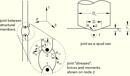
ABAQUS/Standard provides JOINT2D and JOINT3D elements for modeling a joint between structural members or between a structural member and a fixed support. They can be used in an ABAQUS/Aqua analysis to model the interaction between a “spud can” and the sea floor for jack-up foundation analysis in offshore applications.
The joint has two nodes. One of these nodes should be constrained fully (by using a boundary condition) if the joint is between a structural member and a fixed support.
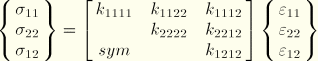
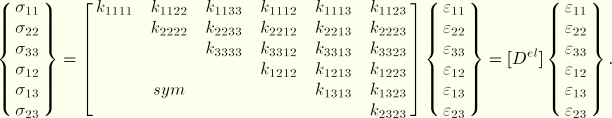
The deformation of the joint is characterized by joint “strains,” which are relative displacements and rotations between the nodes of the joint. The joint must be associated with a user-defined local orientation system (see “Orientations,” Section 2.2.5) that is defined by three orthonormal directions: ![]() ,
, ![]() , and
, and ![]() .
.
The joint, when strained by relative extension or rotation of the two nodes, responds by applying equal and opposite forces and/or moments to the nodes. These forces and moments, or joint “stresses,” can be a linear (elastic) or nonlinear (elastic-plastic) function of the “strains,” depending on the type of constitutive model used in the joint.
The stresses and strains are named as shown in Figure 26.11.1–1. Positive stress indicates tension; positive strain indicates extension.
Even when geometrically nonlinear analysis is requested (“Geometric nonlinearity” in “General and linear perturbation procedures,” Section 6.1.2), the element kinematics are defined with the assumption of small relative displacements and small rotations; therefore, these elements should not be used when these assumptions are violated. If large rotations are required and there is no plasticity, JOINTC elements can be used (see “Flexible joint element,” Section 26.3.1).
The “extensional” strains are defined through
![]()
![]()
![]()
For two-dimensional elements only the axial strains ![]() ,
, ![]() , and the bending strain
, and the bending strain ![]() exist. For three-dimensional elements all six components exist.
exist. For three-dimensional elements all six components exist.
| Input File Usage: | Use the following option to associate a local orientation system with an elastic-plastic joint element: |
*EPJOINT, ORIENTATION=name |
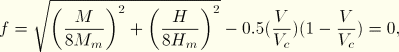
The elastic moduli for joint elasticity can be entered in one of two ways. You can specify a general, anisotropic relation between the forces/moments and elastic extensions. Alternatively, you can enter moduli specific for a spud can; the elastic stiffness matrix is diagonal and depends on the diameter of the spud can at the soil surface, D, which can vary if spud can plasticity is defined and the spud can is conical. See “Joint elasticity models” below for details.
Three joint plasticity models are provided. Two are specific to spud cans. The third is a parabolic model for structural joints or members. See “Joint plasticity” below for details.
If plasticity is included, the plastic straining is assumed to occur in the local 1–2 plane so that the only nonzero plastic strains are ![]() ,
, ![]() , and
, and ![]() . It is assumed that plasticity in the 3-direction can be neglected. In a three-dimensional model strains out of the 1–2 plane produce purely elastic response.
. It is assumed that plasticity in the 3-direction can be neglected. In a three-dimensional model strains out of the 1–2 plane produce purely elastic response.
If the parabolic plasticity model for structural joints or members is used, the 1-direction is the axial direction along the members, while the 2-direction is the transverse direction (see Figure 26.11.1–1). In the spud can plasticity models the 1-direction is the vertical direction, and the 2-direction is the horizontal direction in which plastic extension can take place. In three-dimensional models the 3-direction is the horizontal direction in which only elastic extension can take place.
Any combination of elastic and plastic models can be used. For example, usually spud can elastic moduli will be used with spud can plasticity, but the use of general moduli with spud can plasticity is allowed.
If plasticity is used in a three-dimensional model, coupling is not allowed through the elastic modulus between the strains or stresses in the 1–2 plane (![]() ,
, ![]() ) and the remaining, out-of-plane, strains (
) and the remaining, out-of-plane, strains (![]() ,
, ![]() ). Thus, in this case many of the general elastic moduli must be set to zero.
). Thus, in this case many of the general elastic moduli must be set to zero.
| Input File Usage: | Use one or both of the following options immediately after the related *EPJOINT option to define the joint constitutive model: |
*JOINT ELASTICITY *JOINT PLASTICITY |
Care must be taken in defining the local directions and node numbering so that the motion of node 2 relative to node 1 in the positive 1-direction of the local axis corresponds to extension. Incorrect specification of the local directions or element node numbering can produce incorrect results in plastic analysis because compression will be interpreted as extension.
If one of the nodes must be fixed to represent the ground, it is most convenient to let this node be the first node of the element; extension is then represented by the motion of node 2 of the element in the positive local 1-direction. If a spud can is being modeled in this way, the local 1-direction should be the outward normal to the ocean floor. For a two-dimensional analysis that uses ABAQUS/Aqua structural loads, this direction must be the global y-direction.
For a three-dimensional analysis that uses ABAQUS/Aqua structural loads, the local 1-direction should point in the global z-direction. If plasticity is being used, the local 2-direction should be set so that the 1–2 plane is the plane of greatest deformation.
| Input File Usage: | Use the following orientation definition to model a spud can with the first node fixed: |
*ORIENTATION, NAME=name, TYPE=RECTANGULAR
0, 1, 0, –1, 0, 0
Use the following orientation definition for a three-dimensional ABAQUS/Aqua analysis with plasticity: *ORIENTATION, NAME=name, TYPE=RECTANGULAR 0, 0, 1, x, y, 0 where (x, y, 0) defines the local 2-direction. |
If either spud can elasticity or spud can plasticity is used, you must specify the constants to define the spud can geometry. The entire spud can section definition has no effect if there is neither spud can elasticity nor spud can plasticity.
The spud can, illustrated in Figure 26.11.1–1, can be either conical-based or flat-based. The spud can geometry is defined by ![]() , the diameter of the cylindrical portion, and
, the diameter of the cylindrical portion, and ![]() , the planar angle of the conical portion, where
, the planar angle of the conical portion, where ![]() . You can specify a flat-based spud can by omitting the specification of
. You can specify a flat-based spud can by omitting the specification of ![]() or by giving a value of 0 or 180 for
or by giving a value of 0 or 180 for ![]() .
.
| Input File Usage: | *EPJOINT, SECTION=SPUD CAN |
If spud can plasticity is defined or if there is spud can elasticity and the spud can is conical, you must specify the initial embedment of the spud can, ![]() .
.
The embedment can be prescribed directly or by specifying a “preload” that produces the embedment, as discussed below. Specification of both embedment and preload is not allowed. If either embedment or preload is given, both embedment and equivalent preload (in the case of plasticity) can be examined in the data file at the start of the analysis.
At any time in the analysis the spud can has a total (plastic) embedment of ![]() , where
, where ![]() is the plastic embedment between the start of the analysis and time t. (The negative sign in this equation reflects the fact that the sign convention for strain in ABAQUS is positive for tensile strain. Most often for spud can plasticity,
is the plastic embedment between the start of the analysis and time t. (The negative sign in this equation reflects the fact that the sign convention for strain in ABAQUS is positive for tensile strain. Most often for spud can plasticity, ![]() will be compressive, or negative.) The joint can be purely elastic, in which case
will be compressive, or negative.) The joint can be purely elastic, in which case ![]() , so
, so ![]() always.
always.
The height of the conical portion of the spud can is given by ![]() . The effective diameter of the spud can at the soil surface, D, is defined by
. The effective diameter of the spud can at the soil surface, D, is defined by
For a flat-based spud can:
![]()
For a conical-based spud can:
Cone portion partially penetrating (![]() ):
):
![]()
Penetration beyond cone-cylinder transition (![]() ):
):
![]()
The current spud can area at the soil surface, A, is defined through ![]() . The effective diameter can vary throughout the analysis only for a conical spud can with plasticity.
. The effective diameter can vary throughout the analysis only for a conical spud can with plasticity.
The embedment has no effect and is not required if the spud can is cylindrical and spud can plasticity is not defined.
The embedment value can be prescribed directly using initial conditions (see “Initial conditions,” Section 27.2.1).
| Input File Usage: | *INITIAL CONDITIONS, TYPE=SPUD EMBEDMENT |
If spud can plasticity is defined, you can specify the initial compressive capacity (“preload”), ![]() , instead of the embedment. In this case ABAQUS/Aqua will use the hardening law to calculate the plastic embedment that follows when the preload is applied vertically.
, instead of the embedment. In this case ABAQUS/Aqua will use the hardening law to calculate the plastic embedment that follows when the preload is applied vertically.
The preload initial condition is used only to calculate the initial plastic embedment; the spud can starts the analysis in a zero strain and stress state at this initial plastic embedment, and the preload is assumed to be removed. You must apply any operational vertical load through loading within the history definition.
| Input File Usage: | *INITIAL CONDITIONS, TYPE=SPUD PRELOAD |
Force and moment output in the element local system is available through the “stress” output variable S. Extension and relative rotation are available through the “strain” output variable E. Elastic and plastic strains are available through the output variables EE and PE. For spud cans the plastic embedment since the start of the analysis is available through the vertical component of plastic strain, PE11, and will usually be negative, indicating compression; the total vertical embedment, ![]() , is available through output variable PEEQ. Element nodal force (the force the element places on its nodes, in the global system) is available through element variable NFORC.
, is available through output variable PEEQ. Element nodal force (the force the element places on its nodes, in the global system) is available through element variable NFORC.
The elastic load-displacement behavior of the JOINT2D and JOINT3D elements is characterized by elastic spring stiffnesses, which are assembled to form the elastic element stiffness matrix. A special diagonal modulus for spud cans can be specified or, alternatively, a fully populated (general) elastic modulus can be specified.
Spud can moduli can be prescribed for either two-dimensional or three-dimensional elements.
The elastic stiffness for a two-dimensional spud can is
![]()
is the vertical elastic spring stiffness, ![]() ;
;
![]()
is the horizontal elastic spring stiffness, ![]() ;
;
![]()
is the elastic spring stiffness in bending, ![]() ;
;
| Input File Usage: | *JOINT ELASTICITY, MODULI=SPUD CAN, NDIM=2 |
For a three-dimensional spud can the moduli are
![]()
is the vertical elastic spring stiffness, ![]() ;
;
![]()
is a horizontal elastic spring stiffness, ![]() ;
;
![]()
is a horizontal elastic spring stiffness, ![]() ;
;
![]()
is an elastic spring stiffness in bending, ![]() ;
;
![]()
is an elastic spring stiffness in bending, ![]() ;
;
![]()
is the torsional elastic spring stiffness, ![]() ;
;
Straining out of the 1–2 plane through the strains ![]() , and
, and ![]() produces purely elastic response in the three-dimensional model regardless of plasticity. The moduli related to these strains are assumed not to be affected by the plasticity so that
produces purely elastic response in the three-dimensional model regardless of plasticity. The moduli related to these strains are assumed not to be affected by the plasticity so that ![]() , and
, and ![]() are based on the initial embedded diameter, while the other moduli depend on the current embedded diameter.
are based on the initial embedded diameter, while the other moduli depend on the current embedded diameter.
| Input File Usage: | *JOINT ELASTICITY, MODULI=SPUD CAN, NDIM=3 |
General moduli can be specified for either two-dimensional or three-dimensional elements.
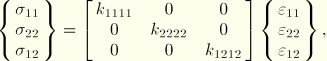
For the two-dimensional case six independent elastic moduli are needed. The stress-strain relations are as follows:
| Input File Usage: | *JOINT ELASTICITY, MODULI=GENERAL, NDIM=2 |
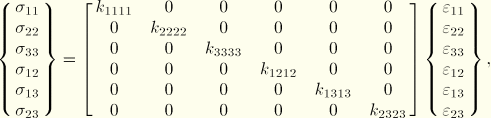
For the three-dimensional case 21 independent elastic moduli are needed. The stress-strain relations are as follows:
| Input File Usage: | *JOINT ELASTICITY, MODULI=GENERAL, NDIM=3 |
In what follows ![]() , and
, and ![]() represent the vertical compressive load, the horizontal load in the 1–2 plane, and the bending moment in the local 1–2 plane, respectively.
represent the vertical compressive load, the horizontal load in the 1–2 plane, and the bending moment in the local 1–2 plane, respectively.
If plasticity is defined, the joint can yield axially, horizontally, or rotationally. The stress depends linearly on the elastic strain. The elastic moduli can depend on the plasticity in the case of a conical spud can, through the diameter at the surface, D.
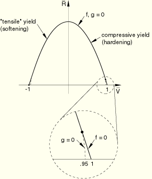
The models are rate independent, with a yield equation of the form
![]()
The flow rule requires that the plastic flow direction is normal to the contours of the flow potential, g. Associated flow is assumed in all of these models (except at vertices in the yield surface, as discussed below).
The three available plasticity models all use parabolic yield surfaces. Each has a compressive and a tensile limit for the stress in the 1-direction, which are termed ![]() and
and ![]() , respectively;
, respectively; ![]() is zero for the clay model. The sign convention for
is zero for the clay model. The sign convention for ![]() and
and ![]() is such that they are always positive; thus,
is such that they are always positive; thus, ![]() always obeys
always obeys
![]()
![]()
![]()
The normalized yield function in ![]() -space for each model is defined through
-space for each model is defined through
![]()
The flow potential is the same as the yield function (associated flow) except that some smoothing is done to the flow potential where the yield function has corners.
The yield surface has corners and, therefore, nonunique normals at points where it is intersected by the ![]() -axis.
-axis.
To avoid problems with the indeterminate flow directions at these corners, ABAQUS/Standard uses a flow potential whose contours are rounded in the region of the vertex, as indicated in the detail of a vertex shown in Figure 26.11.1–2. This rounding is achieved by fitting an elliptical segment to the flow potential contour for ![]() .
.
ABAQUS/Aqua uses fully implicit integration for the plasticity equations. The corresponding tangent stiffness is unsymmetric for these plasticity models. By default, the symmetrized tangent is used in the global Newton loop. If the convergence rate seems to be poor, you may get some benefit out of using the unsymmetric matrix storage and solution scheme for the step (see “Procedures: overview,” Section 6.1.1).
The three models differ only in the definitions of ![]() ,
, ![]() ,
, ![]() , and
, and ![]() and in the hardening definitions. We present the yield function for each model as it is presented in the literature rather than in normalized form. The equivalent normalized form can be obtained by identifying
and in the hardening definitions. We present the yield function for each model as it is presented in the literature rather than in normalized form. The equivalent normalized form can be obtained by identifying ![]() and
and ![]() , which are explicit in the given yield functions for clay and member plasticity; for the sand model they are provided for reference.
, which are explicit in the given yield functions for clay and member plasticity; for the sand model they are provided for reference.
Yield function:
Work hardening equations:
Flat-base spud can:
![]()
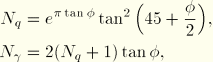
Conical-base spud can:
Cone portion partially penetrating:
![]()
Penetration beyond cone-cylinder transition:
![]()
The constants ![]() and
and ![]() are based on the following empirical relation, which has been derived from centrifuge data:
are based on the following empirical relation, which has been derived from centrifuge data:
![]()
The sand model yield function can be put in normalized form by using ![]() and
and ![]() where
where ![]() . For the model of Osborne et al.
. For the model of Osborne et al. ![]() .
.
This model requires a nonzero initial embedment or equivalent preload.
| Input File Usage: | *JOINT PLASTICITY, TYPE=SAND |
Yield function:
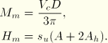
Flat-base spud can:
![]()
Conical-base spud can:
Cone portion penetrating:
![]()
Penetration beyond cone-cylinder transition:
![]()
Work hardening equations:
Flat-base spud can:
![]()
Conical-base spud can:
![]()
This model has zero yield strength in tension ![]() and requires a nonzero initial embedment or equivalent preload.
and requires a nonzero initial embedment or equivalent preload.
| Input File Usage: | *JOINT PLASTICITY, TYPE=CLAY |
Yield function:
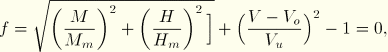
Work hardening: no work hardening is assumed (the model is perfectly plastic).
| Input File Usage: | *JOINT PLASTICITY, TYPE=MEMBER |
Because associated flow is assumed in the spud can plasticity models, tensile vertical plastic strain can occur whenever the yield surface is encountered with ![]() . It is not required that the vertical force itself be tensile for tensile plastic yield to occur; tensile plastic yield can occur on any part of the yield surface where
. It is not required that the vertical force itself be tensile for tensile plastic yield to occur; tensile plastic yield can occur on any part of the yield surface where ![]() . The spud can models soften during this tensile plastic yield; if there is insufficient support from the rest of the model, an instability can occur and the analysis may fail to converge. When this happens, the spud can is likely to be lifting out of the sea floor.
. The spud can models soften during this tensile plastic yield; if there is insufficient support from the rest of the model, an instability can occur and the analysis may fail to converge. When this happens, the spud can is likely to be lifting out of the sea floor.
To make it easier to diagnose analysis problems that may arise due to these issues, a message is printed to the message file in the following cases: if tensile plastic yield occurs for a spud can, if yield occurs near the top of the parabolic yield surface (![]() ) where there is very little hardening, or if the embedment of a spud can becomes less than 10% of the initial embedment. These messages are not printed more than once in a given step.
) where there is very little hardening, or if the embedment of a spud can becomes less than 10% of the initial embedment. These messages are not printed more than once in a given step.
The plasticity algorithm can fail in an iteration if the strain increment is excessively large. Some details that may be of help in diagnosing failure in joint elements can be obtained by requesting detailed printout to the message file of problems with the plasticity algorithms (see “The ABAQUS/Standard message file” in “Output,” Section 4.1.1).