Product: ABAQUS/Standard
A direct cyclic analysis:
is a quasi-static analysis;
uses a combination of Fourier series and time integration of the nonlinear material behavior to obtain the stabilized cyclic response of the structure iteratively;
avoids the considerable numerical expense associated with a transient analysis;
is ideally suited for very large problems in which many load cycles must be applied to obtain the stabilized response if transient analysis is performed;
can be performed with linear or nonlinear material with localized plastic deformation such as when low-cycle fatigue calculations are performed;
can be used to predict the likelihood of plastic ratchetting;
assumes geometrically linear behavior and fixed contact conditions; and
uses the elastic stiffness, so the equation system is inverted only once.
It is well known that after a number of repetitive loading cycles, the response of an elastic-plastic structure, such as an automobile exhaust manifold subjected to large temperature fluctuations and clamping loads, may lead to a stabilized state in which the stress-strain relationship in each successive cycle is the same as in the previous one. The classical approach to obtain the response of such a structure is to apply the periodic loading repetitively to the structure until a stabilized state is obtained. This approach can be quite expensive, since it may require the application of many loading cycles before the stabilized response is obtained. To avoid the considerable numerical expense associated with a transient analysis, a direct cyclic analysis can be used to calculate the cyclic response of the structure directly. The basis of this method is to construct a displacement function ![]() that describes the response of the structure at all times t during a load cycle with period T as shown in Figure 6.2.6–1.
that describes the response of the structure at all times t during a load cycle with period T as shown in Figure 6.2.6–1.
Figure 6.2.6–1 A displacement function at all times t during a load cycle with period T at different iterations.

![]()
![]()
The displacement solution is obtained by solving for corrections to the displacement Fourier coefficients corresponding to each residual coefficient. The updated displacement solution is used in the next iteration to obtain the displacements at each instant in time. This process is repeated until convergence is obtained. Each pass through the complete load cycle can, therefore, be thought of as a single iteration of the solution to the nonlinear problem. Convergence is measured by ensuring that all entries of the residual coefficients are small.
The algorithm to obtain a stabilized cycle is described in detail in “Direct cyclic algorithm,” Section 2.2.3 of the ABAQUS Theory Manual.
A direct cyclic step can be the only step in an analysis, can follow a general or linear perturbation step, or can be followed by a general or linear perturbation step. If a direct cyclic step is followed by a general step, the solution at the end of the direct cyclic step will be the initial state of the general step. If a direct cyclic step follows a general or linear perturbation step, the elastic stiffness matrix at the end of the last general analysis step prior to the direct cyclic step will serve as the Jacobian in the direct cyclic procedure. Any prior (non-cyclic) loads are simply included in the constant part of the Fourier expansion of the residual vectors, and the plastic strains at the end of the preloading step are used as initial conditions for the direct cyclic step.
Multiple direct cyclic analysis steps can be included in a single analysis. In such a case the Fourier series coefficients obtained in the previous step can be used as starting values in the current step. By default, the Fourier coefficients are reset to zero, thus allowing application of cyclic loading conditions that are very different from those defined in the previous direct cyclic step.
You can specify that a direct cyclic step in a restart analysis should use the Fourier coefficients from the previous step, thus allowing continuation of an analysis that has not reached a stabilized cycle. In a direct cyclic analysis a restart file is written at the end of the cycle or time period. Consequently, a restart analysis that is a continuation of a previous direct cyclic analysis will start with a new iteration at ![]() (see “Restarting an analysis,” Section 9.1.1).
(see “Restarting an analysis,” Section 9.1.1).
| Input File Usage: | Use the following option to specify that the current step is a continuation of the previous direct cyclic step: |
*DIRECT CYCLIC, CONTINUE=YES Use the following option to reset the Fourier series coefficients to zero: *DIRECT CYCLIC, CONTINUE=NO (default) |
Direct cyclic analysis combines a Fourier series approximation with time integration of the nonlinear material behavior to obtain the stabilized cyclic solution iteratively using a modified Newton method. The accuracy of the algorithm depends on the number of Fourier terms used, the number of iterations taken to obtain the stabilized solution, and the number of time points within the load period at which the material response and residual vector are evaluated. ABAQUS/Standard allows you to control the solution in several ways, as described below.
In the direct cyclic method global Newton iterations are performed to determine corrections to the displacement Fourier coefficients. During each global iteration ABAQUS/Standard tracks through the entire time cycle to compute the residual vector at a suitable number of time points. This involves standard element-by-element finite element calculations in which history-dependent material variables are integrated. The residual vector is integrated over the period to obtain the Fourier residual coefficients, which in turn yield corrections in displacement coefficients when the system of equations is solved. ABAQUS/Standard will continue with the iterative process until convergence is obtained or until the maximum number of iterations allowed has been reached. You specify the maximum number of iterations when you define the direct cyclic step; the default is 200 iterations.
| Input File Usage: | Use the following option to specify the maximum number of iterations allowed in a direct cyclic step: |
*DIRECT CYCLIC , , , , , , , max number of iterations |
Convergence is best measured by ensuring that all the residual coefficients are sufficiently small compared to the time averaged force and that all the corrections to displacement Fourier coefficients are sufficiently small compared to the displacement Fourier coefficients. The time averaged force is defined in “Convergence criteria for nonlinear problems,” Section 7.2.3. ABAQUS/Standard requires that the ratio of the maximum residual coefficient to the time averaged force, ![]() , and the ratio of the maximum correction to the displacement coefficients to the largest displacement coefficient,
, and the ratio of the maximum correction to the displacement coefficients to the largest displacement coefficient, ![]() , are less than the tolerances. The default values are
, are less than the tolerances. The default values are ![]() = 0.005 and
= 0.005 and ![]() = 0.005. To change these values, you must define direct cyclic controls.
= 0.005. To change these values, you must define direct cyclic controls.
When a stabilized cyclic response does not exist, the method will not converge. In the case where plastic ratchetting occurs, the displacement and residual coefficients on all the periodic terms (![]() , and
, and ![]() ) in the Fourier series converge. However, the displacement and the residual coefficients on the constant term (
) in the Fourier series converge. However, the displacement and the residual coefficients on the constant term (![]() and
and ![]() ) in the Fourier series continue to grow from one iteration to another iteration. The user-specified tolerances
) in the Fourier series continue to grow from one iteration to another iteration. The user-specified tolerances ![]() and
and ![]() are used to detect the plastic ratchetting. The default values are
are used to detect the plastic ratchetting. The default values are ![]() = 0.005 and
= 0.005 and ![]() = 0.005.
= 0.005.
| Input File Usage: | Use the following option to specify the tolerance criteria for direct cyclic convergence: |
*CONTROLS, TYPE=DIRECT CYCLIC |
The number of Fourier terms required to obtain an accurate solution depends on the variation of the load as well as the variation of the structural response over the period. In determining the number of terms, keep in mind that the objective of this kind of analysis is to make low-cycle fatigue predictions. Hence, the goal is to obtain good approximation of the plastic strain cycle at each point; local inaccuracies in the stresses are less important. More Fourier terms usually provide a more accurate solution but at the expense of additional data storage and computational time. In addition, an accurate integration of the Fourier residual coefficients requires that the residual vector be evaluated at an adequate number of time points during the cycle. ABAQUS/Standard uses a trapezoidal rule, which assumes a linear variation of the residual over a time increment, to integrate the residual coefficients. For accurate integration the number of time points must be larger than the number of Fourier coefficients (which is equal to ![]() , where n represents the number of Fourier terms). ABAQUS/Standard will automatically reduce the number of Fourier coefficients used for the next iteration if it is found to be greater than the number of increments taken to complete an iteration.
, where n represents the number of Fourier terms). ABAQUS/Standard will automatically reduce the number of Fourier coefficients used for the next iteration if it is found to be greater than the number of increments taken to complete an iteration.
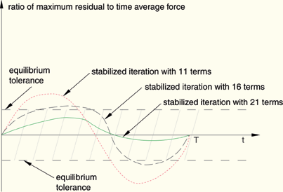
ABAQUS/Standard uses an adaptive algorithm to determine the number of Fourier terms. By default, ABAQUS/Standard starts with 11 terms and determines the response of the structure by using the iterative method described before. Once convergence is obtained (which is measured by ensuring that all the residual vector coefficients and all the corrections to displacement coefficients in the Fourier series are sufficiently small), ABAQUS/Standard evaluates if a sufficient number of Fourier terms are used by determining if equilibrium was satisfied at all the time points during the cycle. If equilibrium is satisfied at all time points, the solution is accepted. Otherwise, ABAQUS/Standard increases the number of Fourier terms (by default, 5 terms are added) and continues with the iterative scheme until convergence with the new number of Fourier terms is obtained. This process is repeated until equilibrium is reached or until the maximum number of Fourier terms has been used. This scheme is best illustrated in Figure 6.2.6–2, where both local equilibrium and overall convergence are obtained when the number of Fourier terms is equal to 21. A maximum number of 25 Fourier terms is used by default. You can specify the initial and maximum number of Fourier terms and the increment in the number of terms when you define the direct cyclic step.
You can also define the convergence criteria for determining convergence and for determining whether equilibrium is achieved at all time points through the period (see “Commonly used control parameters,” Section 7.2.2), with suitable defaults set by ABAQUS/Standard.
In a direct cyclic analysis that has not reached a stabilized cycle, you can increase the number of iterations or Fourier terms upon restart, thus allowing continuation of an analysis.
ABAQUS/Standard provides detailed output of the maximum residual at each time point, the maximum residual coefficient, the maximum displacement coefficient, the maximum correction to displacement coefficients, and the number of Fourier terms at the end of each iteration in the message (.msg) file. This output is described in more detail below.
| Input File Usage: | Use the following option to specify the Fourier series data: |
*DIRECT CYCLIC , , , , initial number of terms, max number of terms, increment in number of terms |
To ensure an accurate solution, the material history as well as the residual vector must be evaluated at a sufficient number of time points during the cycle. The number of time points, ![]() , at which the response is computed must be larger than the number of Fourier coefficients; i.e.,
, at which the response is computed must be larger than the number of Fourier coefficients; i.e., ![]() . ABAQUS/Standard will automatically adjust the number of Fourier coefficients if such a condition is not satisfied. You can specify the time incrementation over the cycle directly, or it can be determined automatically by ABAQUS/Standard.
. ABAQUS/Standard will automatically adjust the number of Fourier coefficients if such a condition is not satisfied. You can specify the time incrementation over the cycle directly, or it can be determined automatically by ABAQUS/Standard.
You should specify the maximum number of increments allowed in the time period as part of the step definition. The default is 100.
There are several ways to choose the automatic incrementation scheme. If you specify only the maximum allowable nodal temperature change in an increment, the time increments are selected automatically based on this value. ABAQUS/Standard will restrict the time increments to ensure that the maximum temperature change is not exceeded at any node during any increment of the analysis.
| Input File Usage: | *DIRECT CYCLIC, DELTMX= |
For rate-dependent constitutive equations you can limit the size of the time increment by the accuracy of the integration. The user-specified accuracy tolerance parameter limits the maximum inelastic strain rate change allowed over an increment:
![]()
| Input File Usage: | *DIRECT CYCLIC, CETOL=tolerance |
If rate-dependent constitutive equations are used in combination with a varying temperature, both controls can be used simultaneously. ABAQUS/Standard will then choose the increments that satisfy both criteria.
| Input File Usage: | *DIRECT CYCLIC, CETOL=tolerance, DELTMX= |
If the time integration accuracy measure specified by either or both of the above controls is satisfied after ![]() consecutive increments without cutbacks, the next time increment will be increased by a factor of
consecutive increments without cutbacks, the next time increment will be increased by a factor of ![]() . Both
. Both ![]() and
and ![]() are user-defined parameters (see “Increasing the time increment size” in “Time integration accuracy in transient problems,” Section 7.2.4). The defaults are
are user-defined parameters (see “Increasing the time increment size” in “Time integration accuracy in transient problems,” Section 7.2.4). The defaults are ![]() = 3 and
= 3 and ![]() = 1.5.
= 1.5.
If neither the accuracy tolerance parameter nor the maximum allowable nodal temperature change is specified, the size of the time increment is fixed. You must specify the time increment ![]() and the time period T.
and the time period T.
| Input File Usage: | *DIRECT CYCLIC |
The user-defined time incrementation for a direct cyclic step can be augmented or superseded by specifying particular time points in the loading history at which the response of the structure should be evaluated. This feature is particularly useful if you know prior to the analysis at which time points in the analysis the load reaches a maximum and/or minimum value or when the response will change rapidly. An example is the analysis of the heating/cooling thermal cycle of an engine component where you typically know when the temperature reaches a maximum value.
When time points are used with fixed time incrementation, the time incrementation specified for the direct cyclic step is ignored and instead the time incrementation precisely follows the specified time points. If time points are used with automatic incrementation, the time incrementation is variable; but the response of the structure will be evaluated at the specified time points.
The time points can be listed individually, or they can be generated automatically by specifying the starting time point, ending time point, and increment in time between the two specified time points.
| Input File Usage: | Use the following options to list time points individually: |
*TIME POINTS, NAME=time points name
*DIRECT CYCLIC, TIME POINTS=time points name
Use the following options to generate time points automatically: *TIME POINTS, NAME=time points name, GENERATE *DIRECT CYCLIC, TIME POINTS=time points name |
By default, ABAQUS/Standard imposes periodic conditions during the iterative solution process by using the state obtained at the end of the previous iteration as the starting state for the current iteration; i.e., ![]() , where s is a solution variable such as plastic strain.
, where s is a solution variable such as plastic strain.
In cases where the periodic solution is not easily found (for example, when the loading is close to causing ratchetting), the state around which the periodic solution is obtained may show considerably more “drift” than would be obtained in a transient analysis. In such cases you may wish to delay the application of periodic conditions as an artificial method to reduce this drift. Figure 6.2.6–3 compares the response of two identical structures subjected to the same set of cyclic loads and boundary conditions, where each structure experienced a different loading history prior to the application of the cyclic loads. Figure 6.2.6–3 shows that the prior loading history only affects the mean value of stress and strain; it does not affect the shape of the stress-strain curves or the amount of energy dissipated during the cycle.
Figure 6.2.6–3 Influence of periodicity condition on mean value of the strains over a stabilized cycle.

You can control when the periodicity conditions are applied by defining direct cyclic controls to specify the variable ![]() . This variable defines from which iteration onward the application of periodic conditions will be activated. For example, setting
. This variable defines from which iteration onward the application of periodic conditions will be activated. For example, setting ![]() means that the periodicity conditions are applied from iteration 6 onwards. The default is
means that the periodicity conditions are applied from iteration 6 onwards. The default is ![]() , which is appropriate for most analyses.
, which is appropriate for most analyses.
| Input File Usage: | Use the following option to specify the iteration number at which the periodicity condition is first imposed: |
*CONTROLS, TYPE=DIRECT CYCLIC |
Initial values of stresses, temperatures, field variables, solution-dependent state variables, etc. can be specified (see “Initial conditions,” Section 27.2.1).
Boundary conditions can be applied to any of the displacement or rotation degrees of freedom. During the analysis, prescribed boundary conditions must have an amplitude definition that is cyclic over the step: the start value must be equal to the end value (see “Amplitude curves,” Section 27.1.2). If the analysis consists of several steps, the usual rules apply (see “Boundary conditions,” Section 27.3.1). At each new step the boundary condition can either be modified or completely defined. All boundary conditions defined in previous steps remain unchanged unless they are redefined.
The following loads can be prescribed in a direct cyclic analysis:
Concentrated nodal forces can be applied to the displacement degrees of freedom (1–6); see “Concentrated loads,” Section 27.4.2.
Distributed pressure forces or body forces can be applied; see “Distributed loads,” Section 27.4.3. The distributed load types available with particular elements are described in Part VI, “Elements.”
The following predefined fields can be specified in a direct cyclic analysis, as described in “Predefined fields,” Section 27.6.1:
Temperature is not a degree of freedom in a direct cyclic analysis, but nodal temperatures can be specified as a predefined field. The temperature values specified must be cyclic over the step: the start value must be equal to the end value (see “Amplitude curves,” Section 27.1.2). If the temperatures are read from the results file, you should specify initial temperature conditions equal to the temperature values at the end of the step (see “Initial conditions,” Section 27.2.1). Alternatively, you can ramp the temperatures back to their initial condition values, as described in “Predefined fields,” Section 27.6.1. Any difference between the applied and initial temperatures will cause thermal strain if a thermal expansion coefficient is given for the material (“Thermal expansion,” Section 20.1.2). The specified temperature also affects temperature-dependent material properties, if any.
The values of user-defined field variables can be specified. These values affect only field-variable-dependent material properties, if any. The field variable values specified must be cyclic over the step.
Most material models, including user-defined materials (defined using user subroutine UMAT), that describe mechanical behavior are available for use in a direct cyclic analysis.
The following material properties are not active during a direct cyclic analysis: acoustic properties, thermal properties (except for thermal expansion), mass diffusion properties, electrical conductivity properties, piezoeletric properties, and pore fluid flow properties.
Rate-dependent yield (“Rate-dependent yield,” Section 18.2.3), rate-dependent creep (“Rate-dependent plasticity: creep and swelling,” Section 18.2.4), and two-layer viscoplasticity (“Two-layer viscoplasticity,” Section 18.2.11) can also be used during a direct cyclic analysis.
Any of the stress/displacement elements in ABAQUS/Standard can be used in a direct cyclic analysis (see “Choosing the appropriate element for an analysis type,” Section 21.1.3).
Different types of output are available for postprocessing and for monitoring a direct cyclic analysis.
ABAQUS/Standard prints the residual force, time average force, and a flag to indicate if equilibrium was satisfied in the message (.msg) file at different time increments for each iteration. You can control the frequency in increments at which information is printed to the message file, and you can suppress the output; the default is to print output every 10 increments (see “The ABAQUS/Standard message file” in “Output,” Section 4.1.1, for more information).
ABAQUS/Standard also prints the number of Fourier terms used, the maximum residual coefficient, the maximum correction to displacement coefficients, and the maximum displacement coefficient in the Fourier series in the message file at the end of each iteration. An example of the output is shown below:
 									           ITERATION    26 STARTS
 INC     TIME        STEP       LARG. RESI.   TIME AVG.   FORCE
         INC         TIME       FORCE         FORCE       EQUV.
 10      0.250       2.50       1.008E+01     50.9         N
 20      0.250       5.00       1.622E+01     76.8         N
 30      0.250       7.50       4.622E-02     99.8         Y

                     ITERATION    26 SUMMARY
 NUMBER OF FOURIER TERMS USED 40, TOTAL NUMBER OF INCREMENTS  120
 CYCLE/STEP TIME   30.0,    TOTAL TIME COMPLETED       31.0
 AVERAGE FORCE     21.2     TIME AVG. FORCE     25.7

 MAX. COEFFICIENT OF DISP.                   0.142  AT NODE 24 DOF 2
 MAX. COEFF. OF RESI. FORCE ON CONST. TERM    31.7  AT NODE 44 DOF 1
 MAX. COEFF. OF RESI. FORCE ON PERI. TERMS    0.82  AT NODE  6 DOF 3
 MAX. CORR. TO COEFF. OF DISP. ON CONST. TERM 0.002 AT NODE 50 DOF 3
MAX. CORR. TO COEFF. OF DISP. ON PERI. TERMS 0.015 AT NODE 50 DOF 3Element and nodal output are written only when the stabilized cycle is reached. If a stabilized cycle has not been reached at the end of an analysis, output is written for the last iteration of the step. The element output available for a direct cyclic analysis includes stress; strain; energies; and the values of state, field, and user-defined variables. All the energies are set equal to zero at the beginning of each iteration since energies dissipated over an entire stabilized cycle are of interest in making fatigue life predictions in direct cyclic analysis. The nodal output available includes displacements, reaction forces, and coordinates. All of the output variable identifiers are outlined in “ABAQUS/Standard output variable identifiers,” Section 4.2.1.
You may want to recover additional results for an iteration rather than for the stabilized cycle. You can extract these results from the restart data (see “Output,” Section 4.1.1). This feature is particularly useful if you want to evaluate the shift of the strain from one iteration to another iteration when plastic ratchetting occurs.
| Input File Usage: | *POST OUTPUT, ITERATION=n |
A direct cyclic analysis is subject to the following limitations:
Contact conditions cannot change during a direct cyclic analysis; they remain as they were defined at the beginning of the analysis or at the end of any general step prior to the direct cyclic step. Frictional slipping is not allowed during direct cyclic analyses; all points in contact are assumed to be sticking if friction is present.
Geometric nonlinearity can be included only in any general step prior to a direct cyclic step; however, only small displacements and strains will be considered during the cyclic step.
*HEADING
…
*BOUNDARY
Data lines to specify zero-valued boundary conditions
*INITIAL CONDITIONS
Data lines to specify initial conditions
*AMPLITUDE
Data lines to define amplitude variations
**
*STEP (,INC=)
Set  INC equal to the maximum number of increments in a single loading cycle
*DIRECT CYCLIC
Data line to define time increment, cycle time, initial number of Fourier terms,
maximum number of Fourier terms, increment in number of Fourier terms,
and maximum number of iterations
*TIME POINTS
Data lines to list time points
*BOUNDARY, AMP=
Data lines to prescribe zero-valued or nonzero boundary conditions
*CLOAD and/or *DLOAD, AMP=
Data lines to specify loads
*TEMPERATURE and/or *FIELD, AMP=
Data lines to specify values of predefined fields
*END STEP
**
*STEP(,INC=)
*DIRECT CYCLIC, DELTMX
Data line to control automatic time incrementation and Fourier representations
*BOUNDARY, OP=MOD,AMP=
Data lines to modify or add zero-valued or nonzero boundary conditions
*CLOAD, OP=NEW, AMP=
Data lines to specify new concentrated loads; all previous concentrated
loads will be removed
*DLOAD, OP=MOD, AMP=
Data lines to specify additional or modified distributed loads
*TEMPERATURE and/or *FIELD, AMP=
Data lines to specify additional or modified values of predefined fields
*END STEP