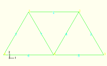
This example of an overhead hoist, shown in Figure 2–5, leads you through the ABAQUS/CAE modeling process by using the Model Tree and showing you the basic steps used to create and analyze a simple model. The hoist is a simple, pin-jointed framework that is constrained at the left end and mounted on rollers at the right end. The members can rotate freely at the joints. The frame is prevented from moving out of plane. A simulation is first performed in ABAQUS/Standard to determine the structure's static deflection and the peak stress in its members when a 10 kN load is applied as shown in Figure 2–5. The simulation is performed a second time in ABAQUS/Explicit under the assumption that the load is applied suddenly to study the dynamic response of the frame.
For the overhead hoist example, you will perform the following tasks:
Sketch the two-dimensional geometry and create a part representing the frame.
Define the material properties and section properties of the frame.
Assemble the model.
Configure the analysis procedure and output requests.
Apply loads and boundary conditions to the frame.
Mesh the frame.
Create a job and submit it for analysis.
View the results of the analysis.
A Python script for this example is provided in “Overhead hoist frame,” Section A.1. When this script is run in ABAQUS/CAE, it creates the complete analysis model for this problem. Run the script if you encounter difficulties following the instructions given below or if you wish to check your work. Instructions on how to fetch and run the script are given in Appendix A, “Example Files.”
As noted earlier, it is assumed that you will be using ABAQUS/CAE to generate the model. However, if you do not have access to ABAQUS/CAE or another preprocessor, the input file that defines this problem can be created manually, as discussed in “Creating an input file,” Section 2.3 of Getting Started with ABAQUS/Standard: Keywords Version.
Before starting to define this or any model, you need to decide which system of units you will use. ABAQUS has no built-in system of units. Do not include unit names or labels when entering data in ABAQUS. All input data must be specified in consistent units. Some common systems of consistent units are shown in Table 2–1.
| Quantity | SI | SI (mm) | US Unit (ft) | US Unit (inch) |
|---|---|---|---|---|
| Length | m | mm | ft | in |
| Force | N | N | lbf | lbf |
| Mass | kg | tonne (103 kg) | slug | lbf s2/in |
| Time | s | s | s | s |
| Stress | Pa (N/m2) | MPa (N/mm2) | lbf/ft2 | psi (lbf/in2) |
| Energy | J | mJ (10–3 J) | ft lbf | in lbf |
| Density | kg/m3 | tonne/mm3 | slug/ft3 | lbf s2/in4 |
The SI system of units is used throughout this guide. Users working in the systems labeled “US Unit” should be careful with the units of density; often the densities given in handbooks of material properties are multiplied by the acceleration due to gravity.
Parts define the geometry of the individual components of your model and, therefore, are the building blocks of an ABAQUS/CAE model. You can create parts that are native to ABAQUS/CAE, or you can import parts created by other applications either as a geometric representation or as a finite element mesh.
You will start the overhead hoist problem by creating a two-dimensional, deformable wire part. You do this by sketching the geometry of the frame. ABAQUS/CAE automatically enters the Sketcher when you create a part.
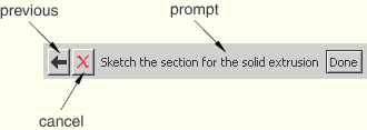
ABAQUS/CAE often displays a short message in the prompt area indicating what you should do next, as shown in Figure 2–6.
Click the Cancel button to cancel the current task. Click the Previous button to cancel the current step in the task and return to the previous step.To create the overhead hoist frame:
If you did not already start ABAQUS/CAE, type abaqus cae, where abaqus is the command used to run ABAQUS.
Select Create Model Database from the Start Session dialog box that appears.
ABAQUS/CAE enters the Part module. The Model Tree appears in the left side of the main window (underneath the Model tab). Between the Model Tree and the canvas is the Part module toolbox. A toolbox contains a set of icons that allow expert users to bypass the menus in the main menu bar. For many tools, as you select an item from the main menu bar or the Model Tree, the corresponding tool is highlighted in the module toolbox so you can learn its location.
In the Model Tree, double-click the Parts container to create a new part.
The Create Part dialog box appears. ABAQUS/CAE also displays text in the prompt area near the bottom of the window to guide you through the procedure.
You use the Create Part dialog box to name the part; to choose its modeling space, type, and base feature; and to set the approximate size. You can edit and rename a part after you create it; you can also change its modeling space and type but not its base feature.
Name the part Frame. Choose a two-dimensional planar deformable body and a wire base feature.
In the Approximate size text field, type 4.0.
The value entered in the Approximate size text field at the bottom of the dialog box sets the approximate size of the new part. The size that you enter is used by ABAQUS/CAE to calculate the size of the Sketcher sheet and the spacing of its grid. You should choose this value to be on the order of the largest dimension of your finished part. Recall that ABAQUS/CAE does not use specific units, but the units must be consistent throughout the model. In this model SI units will be used.
Click Continue to exit the Create Part dialog box.
ABAQUS/CAE automatically enters the Sketcher. The Sketcher toolbox appears in the left side of the main window, and the Sketcher grid appears in the viewport. The Sketcher contains a set of basic tools that allow you to sketch the two-dimensional profile of your part. ABAQUS/CAE enters the Sketcher whenever you create or edit a part. To finish using any tool, click mouse button 2 in the viewport or select a new tool.
Tip: Like all tools in ABAQUS/CAE, if you simply position the cursor over a tool in the Sketcher toolbox for a short time, a small window appears that gives a brief description of the tool. When you select a tool, a white background appears on it.
The following aspects of the Sketcher help you sketch the desired geometry:
The Sketcher grid helps you position the cursor and align objects in the viewport.
Dashed lines indicate the X- and Y-axes of the sketch and intersect at the origin of the sketch.
A triad in the lower-left corner of the viewport indicates the relationship between the sketch plane and the orientation of the part.
When you select a sketching tool, ABAQUS/CAE displays the X- and Y-coordinates of the cursor in the upper-left corner of the viewport.
You will first sketch a rough approximation of the frame and later use constraints and dimensions to refine the sketch. Begin by using the Create Lines: Rectangle tool ![]() located in the upper-right region of the Sketcher toolbox to sketch an arbitrary rectangle. Select any two points as the opposite corners of the rectangle.
located in the upper-right region of the Sketcher toolbox to sketch an arbitrary rectangle. Select any two points as the opposite corners of the rectangle.
Click mouse button 2 anywhere in the viewport to exit the rectangle tool.
Note:
If you make a mistake while using the Sketcher, you can undo your last action using the Undo tool ![]() or delete individual entities of your sketch using the Delete tool
or delete individual entities of your sketch using the Delete tool ![]() .
.
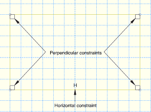
The Sketcher automatically adds constraints to the sketch as indicated in Figure 2–7 (in this case, the four corners of the rectangle are assigned perpendicular constraints and one edge is designated as horizontal).
To proceed, the perpendicular constraints must be deleted. In the Sketcher toolbox, select the Delete toolIn the prompt area, select Constraints as the scope of the operation.
Using [Shift]+Click, select the four perpendicular constraints.
Click Done in the prompt area.
You will now add additional constraints and dimensions to refine the sketch. Constraints and dimensions allow you to control your sketch geometry and add precision. For more information on constraints and dimensions, see “Controlling sketch geometry,” Section 19.7 of the ABAQUS/CAE User's Manual.
Use the Add Constraint tool ![]() to constrain the top and bottom edges so they remain parallel to each other:
to constrain the top and bottom edges so they remain parallel to each other:
In the Add Constraint dialog box, select Parallel.
In the viewport, select the top and bottom edges of the sketch (using [Shift]+Click).
Click Done in the prompt area.
Use the Add Dimension tool ![]() to dimension the top and bottom edges of the rectangle. The top edge should have a horizontal dimension of 1 m and the bottom edge a horizontal dimension of 2 m. When dimensioning each edge, simply select the line, click mouse button 1 to position the dimension text, and then enter the new dimension in the prompt area. Selecting the line rather than its endpoints constrains the length of the line regardless of its orientation in space (in effect, defining an oblique dimension).
to dimension the top and bottom edges of the rectangle. The top edge should have a horizontal dimension of 1 m and the bottom edge a horizontal dimension of 2 m. When dimensioning each edge, simply select the line, click mouse button 1 to position the dimension text, and then enter the new dimension in the prompt area. Selecting the line rather than its endpoints constrains the length of the line regardless of its orientation in space (in effect, defining an oblique dimension).
Reset the view as needed using the Auto-Fit View tool ![]() in the toolbar to see the updated sketch.
in the toolbar to see the updated sketch.
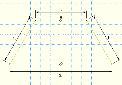
Dimension the left and right edges so they each have an oblique dimension of 1 m.
The sketch in its current state is shown in Figure 2–8. In this figure, every other grid line has been suppressed for visibility. For information on using the Sketcher Options tool ![]() to modify the Sketcher display, see “Customizing the Sketcher,” Section 19.9 of the ABAQUS/CAE User's Manual.
to modify the Sketcher display, see “Customizing the Sketcher,” Section 19.9 of the ABAQUS/CAE User's Manual.
Now sketch the interior edges of the frame.
Using the Create Lines: Connected tool ![]() located in the upper-right corner of the Sketcher toolbox, create two lines as follows:
located in the upper-right corner of the Sketcher toolbox, create two lines as follows:
Start the first line at the upper-left corner of the sketch and extend it to any point that snaps onto the bottom edge (its horizontal location is arbitrary).
Continue the second line to the upper-right corner of the sketch.
Click mouse button 2 anywhere in the viewport to exit the connected lines tool.
Using the Split tool ![]() , split the bottom edge at the point where it intersects the two lines created above:
, split the bottom edge at the point where it intersects the two lines created above:
Note the small black triangles at the base of some of the toolbox icons. These triangles indicate the presence of hidden icons that can be revealed. Click the Auto-Trim tool ![]() located on the middle-right of the Sketcher toolbox, but do not release mouse button 1. Additional icons appear.
located on the middle-right of the Sketcher toolbox, but do not release mouse button 1. Additional icons appear.
Without releasing mouse button 1, drag the cursor along the set of icons that appear until you reach the split tool ![]() . Then release the mouse button to select that tool.
. Then release the mouse button to select that tool.
The split tool appears in the Sketcher toolbox with a white background indicating that you selected it.
Select the bottom edge as the first entity to define the split point.
Select either of the two interior lines as the second entity (a red circle will appear around the split point).
Use the Add Constraint tool ![]() to constrain the two segments of the bottom edge so they are of equal length:
to constrain the two segments of the bottom edge so they are of equal length:
In the Add Constraint dialog box, select Equal length.
In the viewport, select the two segments of the bottom edge.
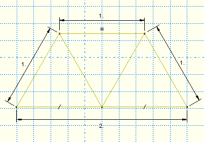
Click Done in the prompt area.
The final sketch is shown in Figure 2–9.
From the prompt area (near the bottom of the main window), click Done to exit the Sketcher.
Note: If you don't see the Done button in the prompt area, continue to click mouse button 2 in the viewport until it appears.
Before you continue, save your model in a model database file.
From the main menu bar, select File![]() Save. The Save Model Database As dialog box appears.
Save. The Save Model Database As dialog box appears.
Type a name for the new model database in the File Name field, and click OK. You do not need to include the file extension; ABAQUS/CAE automatically appends .cae to the file name.
ABAQUS/CAE stores the model database in a new file and returns to the Part module. The path and name of your model database appear in the main window title bar.
You should always save your model database at regular intervals (for example, each time you switch modules); ABAQUS/CAE does not save your model database automatically.
In this problem all the members of the frame are made of steel and assumed to be linear elastic with Young's modulus of 200 GPa and Poisson's ratio of 0.3. Thus, you will create a single linear elastic material with these properties.
To define a material:
In the Model Tree, double-click the Materials container to create a new material.
ABAQUS/CAE switches to the Property module, and the Edit Material dialog box appears.
Name the material Steel.
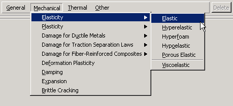
Use the menu bar under the browser area of the material editor to reveal menus containing all the available material options. Some of the menu items contain submenus; for example, Figure 2–10 shows the options available under the Mechanical![]() Elasticity menu item. When you select a material option, the appropriate data entry form appears below the menu.
Elasticity menu item. When you select a material option, the appropriate data entry form appears below the menu.
From the material editor's menu bar, select Mechanical![]() Elasticity
Elasticity![]() Elastic.
Elastic.
ABAQUS/CAE displays the Elastic data form.
Type a value of 200.0E9 for Young's modulus and a value of 0.3 for Poisson's ratio in the respective fields. Use [Tab] or move the cursor to a new cell and click to move between cells.
Click OK to exit the material editor.
You define the properties of a part through sections. After you create a section, you can use one of the following two methods to assign the section to the part in the current viewport:
You can simply select the region from the part and assign the section to the selected region.
You can use the Set toolset to create a homogeneous set containing the region and assign the section to the set.
Defining a truss section
A truss section definition requires only a material reference and the cross-sectional area. Remember that the frame members are circular bars that are 0.005 m in diameter. Thus, their cross-sectional area is 1.963 × 10⁻⁵ m2.
Tip:
You can use the command line interface (CLI) in ABAQUS/CAE as a simple calculator. For example, to compute the cross-sectional area of the frame members, click the ![]() tab in the bottom left corner of the ABAQUS/CAE window to activate the CLI, type 3.1416*0.005**2/4.0 after the command prompt, and press [Enter]. The value of the cross-sectional area is printed in the CLI.
tab in the bottom left corner of the ABAQUS/CAE window to activate the CLI, type 3.1416*0.005**2/4.0 after the command prompt, and press [Enter]. The value of the cross-sectional area is printed in the CLI.
To define a truss section:
In the Model Tree, double-click the Sections container to create a section.
The Create Section dialog box appears.
In the Create Section dialog box:
Name the section FrameSection.
In the Category list, select Beam.
In the Type list, select Truss.
Click Continue.
The Edit Section dialog box appears.
In the Edit Section dialog box:
Accept the default selection of Steel for the Material associated with the section. If you had defined other materials, you could click the arrow next to the Material text box to see a list of available materials and to select the material of your choice.
In the Cross-sectional area field, enter a value of 1.963E-5 (or copy and paste the value from the CLI if you followed the steps outlined in the tip).
Click OK.
Assigning the section to the frame
The section FrameSection must be assigned to the frame.
To assign the section to the frame:
In the Model Tree, expand the branch for the part named Frame by clicking the “![]() ” symbol to expand the Parts container and then clicking the “
” symbol to expand the Parts container and then clicking the “![]() ” symbol to expand the Frame item.
” symbol to expand the Frame item.
Double-click Section Assignments in the list of part attributes that appears.
ABAQUS/CAE displays prompts in the prompt area to guide you through the procedure.
Select the entire part as the region to which the section will be applied.
Click and hold mouse button 1 at the upper left-hand corner of the viewport.
Drag the mouse to create a box around the truss.
Release mouse button 1.
ABAQUS/CAE highlights the entire frame.
Click mouse button 2 in the viewport or click Done in the prompt area to accept the selected geometry.
The Edit Section Assignment dialog box appears containing a list of existing sections.
Accept the default selection of FrameSection, and click OK.
ABAQUS/CAE assigns the truss section to the frame, colors the entire frame aqua to indicate that the region has a section assignment, and closes the Edit Section Assignment dialog box.
Each part that you create is oriented in its own coordinate system and is independent of the other parts in the model. Although a model may contain many parts, it contains only one assembly. You define the geometry of the assembly by creating instances of a part and then positioning the instances relative to each other in a global coordinate system. An instance may be independent or dependent. Independent part instances are meshed individually, while the mesh of a dependent part instance is associated with the mesh of the original part. For further details, see “Working with part instances,” Section 13.3 of the ABAQUS/CAE User's Manual. By default, part instances are dependent.
For this problem you will create a single instance of your overhead hoist. ABAQUS/CAE positions the instance so that the origin of the sketch that defined the frame overlays the origin of the assembly's default coordinate system.
To define the assembly:
In the Model Tree, expand the Assembly container and double-click Instances in the list that appears.
ABAQUS/CAE switches to the Assembly module, and the Create Instance dialog box appears.
In the dialog box, select Frame and click OK.
ABAQUS/CAE creates an instance of the overhead hoist. In this example the single instance of the frame defines the assembly. The frame is displayed in the 1–2 plane of the global coordinate system (a right-handed, rectangular Cartesian system). A triad in the lower-left corner of the viewport indicates the orientation of the model with respect to the view. A second triad in the viewport indicates the origin and orientation of the global coordinate system (X-, Y-, and Z-axes). The global 1-axis is the horizontal axis of the hoist, the global 2-axis is the vertical axis, and the global 3-axis is normal to the plane of the framework. For two-dimensional problems such as this one ABAQUS requires that the model lie in a plane parallel to the global 1–2 plane.
Now that you have created your assembly, you can configure your analysis. In this simulation we are interested in the static response of the overhead hoist to a 10 kN load applied at the center, with the left-hand end fully constrained and a roller constraint on the right-hand end (see Figure 2–5). This is a single event, so only a single analysis step is needed for the simulation. Thus, the model will consist of two steps overall:
An initial step, in which you will apply boundary conditions that constrain the ends of the frame.
An analysis step, in which you will apply a concentrated load at the center of the frame.
There are two kinds of analysis steps in ABAQUS: general analysis steps, which can be used to analyze linear or nonlinear response, and linear perturbation steps, which can be used only to analyze linear problems. Only general analysis steps are available in ABAQUS/Explicit. For this simulation you will define a static linear perturbation step. Perturbation procedures are discussed further in Chapter 11, “Multiple Step Analysis.”
Creating an analysis step
Create a static, linear perturbation step that follows the initial step of the analysis.
To create a static linear perturbation analysis step:
In the Model Tree, double-click the Steps container to create a step.
ABAQUS/CAE switches to the Step module, and the Create Step dialog box appears. A list of all the general procedures and a default step name of Step-1 is provided.
Change the step name to Apply load.
Select Linear perturbation as the Procedure type.
From the list of available linear perturbation procedures in the Create Step dialog box, select Static, Linear perturbation and click Continue.
The Edit Step dialog box appears with the default settings for a static linear perturbation step.
The Basic tab is selected by default. In the Description field, type 10 kN central load.
Click the Other tab to see its contents; you can accept the default values provided for the step.
Click OK to create the step and to exit the Edit Step dialog box.
Requesting data output
Finite element analyses can create very large amounts of output. ABAQUS allows you to control and manage this output so that only data required to interpret the results of your simulation are produced. Four types of output are available from an ABAQUS analysis:
Results stored in a neutral binary file used by ABAQUS/CAE for postprocessing. This file is called the ABAQUS output database file and has the extension .odb.
Printed tables of results, written to the ABAQUS data (.dat) file. Output to the data file is available only in ABAQUS/Standard.
Restart data used to continue the analysis, written to the ABAQUS restart (.res) file.
Results stored in binary files for subsequent postprocessing with third-party software, written to the ABAQUS results (.fil) file.
By default, ABAQUS/CAE writes the results of the analysis to the output database (.odb) file. When you create a step, ABAQUS/CAE generates a default output request for the step. A list of the preselected variables written by default to the output database is given in the ABAQUS Analysis User's Manual. You do not need to do anything to accept these defaults. You use the Field Output Requests Manager to request output of variables that should be written at relatively low frequencies to the output database from the entire model or from a large portion of the model. You use the History Output Requests Manager to request output of variables that should be written to the output database at a high frequency from a small portion of the model; for example, the displacement of a single node.
For this example you will examine the output requests to the .odb file and accept the default configuration.
To examine your output requests to the .odb file:
In the Model Tree, click mouse button 3 on the Field Output Requests container and select Manager from the menu that appears.
ABAQUS/CAE displays the Field Output Requests Manager. This manager displays the status of field output requests in a table format. The left side of the table has an alphabetical list of existing output requests. The top of the table lists the names of all the steps in the analysis in the order of execution. Each cell of the table displays the status of each output request in each step.
You can use the Field Output Requests Manager to do the following:
Select the variables that ABAQUS will write to the output database.
Select the section points for which ABAQUS will generate output data.
Select the region of the model for which ABAQUS will generate output data.
Change the frequency at which ABAQUS will write data to the output database.
Review the default output request that ABAQUS/CAE generates for the Static, Linear perturbation step you created and named Apply load.
Click the cell in the table labeled Created; that cell becomes highlighted. The following information related to the cell is shown in the legend at the bottom of the manager:
The type of analysis procedure carried out in the step in that column.
The list of output request variables.
The output request status.
On the right side of the Field Output Requests Manager, click Edit to view more detailed information about the output request.
The field output editor appears. In the Output Variables region of this dialog box, there is a text box that lists all variables that will be output. If you change an output request, you can always return to the default settings by clicking Preselected defaults above the text box.
Click the arrows next to each output variable category to see exactly which variables will be output. The boxes next to each category title allow you to see at a glance whether all variables in that category will be output. A black check mark indicates that all variables are output, while a gray check mark indicates that only some variables will be output.
Based on the selections shown at the bottom of the dialog box, data will be generated at every default section point in the model and will be written to the output database after every increment during the analysis.
Click Cancel to close the field output editor, since you do not wish to make any changes to the default output requests.
Click Dismiss to close the Field Output Requests Manager.
Note: What is the difference between the Dismiss and Cancel buttons? Dismiss buttons appear in dialog boxes that contain data that you cannot modify. For example, the Field Output Requests Manager allows you to view output requests, but you must use the field output editor to modify those requests. Clicking the Dismiss button simply closes the Field Output Requests Manager. Conversely, Cancel buttons appear in dialog boxes that allow you to make changes. Clicking Cancel closes the dialog box without saving your changes.
Review the history output requests in a similar manner by right-clicking the History Output Requests container in the Model Tree and opening the history output editor.
Prescribed conditions, such as loads and boundary conditions, are step dependent, which means that you must specify the step or steps in which they become active. Now that you have defined the steps in the analysis, you can define prescribed conditions.
Applying boundary conditions to the frame
In structural analyses, boundary conditions are applied to those regions of the model where the displacements and/or rotations are known. Such regions may be constrained to remain fixed (have zero displacement and/or rotation) during the simulation or may have specified, nonzero displacements and/or rotations.
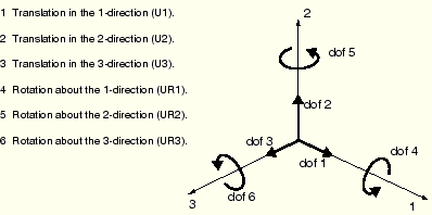
In this model the bottom-left portion of the frame is constrained completely and, thus, cannot move in any direction. The bottom-right portion of the frame, however, is fixed in the vertical direction but is free to move in the horizontal direction. The directions in which motion is possible are called degrees of freedom (dof).
The labeling convention used for the displacement and rotational degrees of freedom in ABAQUS is shown in Figure 2–11.
To apply boundary conditions to the frame:
In the Model Tree, double-click the BCs container.
ABAQUS/CAE switches to the Load module, and the Create Boundary Condition dialog box appears.
In the Create Boundary Condition dialog box:
Name the boundary condition Fixed.
From the list of steps, select Initial as the step in which the boundary condition will be activated. All the mechanical boundary conditions specified in the Initial step must have zero magnitudes. This condition is enforced automatically by ABAQUS/CAE.
In the Category list, accept Mechanical as the default category selection.
In the Types for Selected Step list, select Displacement/Rotation, and click Continue.
ABAQUS/CAE displays prompts in the prompt area to guide you through the procedure. For example, you are asked to select the region to which the boundary condition will be applied.
To apply a prescribed condition to a region, you can either select the region directly in the viewport or apply the condition to an existing set (a set is a named region of a model). Sets are a convenient tool that can be used to manage large complicated models. In this simple model you will not make use of sets.
In the viewport, select the vertex at the bottom-left corner of the frame as the region to which the boundary condition will be applied.
Click mouse button 2 in the viewport or click Done in the prompt area to indicate that you have finished selecting regions.
The Edit Boundary Condition dialog box appears. When you are defining a boundary condition in the initial step, all available degrees of freedom are unconstrained by default.
In the dialog box:
Toggle on U1 and U2 since all translational degrees of freedom need to be constrained.
Click OK to create the boundary condition and to close the dialog box.
ABAQUS/CAE displays two arrowheads at the vertex to indicate the constrained degrees of freedom.
Repeat the above procedure to constrain degree of freedom U2 at the vertex at the bottom-right corner of the frame. Name this boundary condition Roller.
In the Model Tree, click mouse button 3 on the BCs container and select Manager from the menu that appears.
ABAQUS/CAE displays the Boundary Condition Manager. The manager indicates that the boundary conditions are Created (activated) in the initial step and are Propagated from base state (continue to be active) in the analysis step Apply load.
Tip: To view the title of a column in its entirety, expand its width by dragging the dividing line between the column headings.
Click Dismiss to close the Boundary Condition Manager.
In this example all the constraints are in the global 1- or 2-directions. In many cases constraints are required in directions that are not aligned with the global directions. In such cases you can define a local coordinate system for boundary condition application. The skew plate example in Chapter 5, “Using Shell Elements,” demonstrates how to do this.
Applying a load to the frame
Now that you have constrained the frame, you can apply a load to the bottom of the frame. In ABAQUS the term load (as in the Load module in ABAQUS/CAE) generally refers to anything that induces a change in the response of a structure from its initial state, including:
concentrated forces,
pressures,
nonzero boundary conditions,
body loads, and
temperature (with thermal expansion of the material defined).
In this simulation a concentrated force of 10 kN is applied in the negative 2-direction to the bottom center of the frame; the load is applied during the linear perturbation step you created earlier. In reality there is no such thing as a concentrated, or point, load; the load will always be applied over some finite area. However, if the area being loaded is small, it is an appropriate idealization to treat the load as a concentrated load.
To apply a concentrated force to the frame:
In the Model Tree, click mouse button 3 on the Loads container and select Manager from the menu that appears.
The Load Manager appears.
At the bottom of the Load Manager, click Create.
The Create Load dialog box appears.
In the Create Load dialog box:
Name the load Force.
From the list of steps, select Apply load as the step in which the load will be applied.
In the Category list, accept Mechanical as the default category selection.
In the Types for Selected Step list, accept the default selection of Concentrated force.
Click Continue.
ABAQUS/CAE displays prompts in the prompt area to guide you through the procedure. You are asked to select a region to which the load will be applied.
As with boundary conditions, the region to which the load will be applied can be selected either directly in the viewport or from a list of existing sets. As before, you will select the region directly in the viewport.
In the viewport, select the vertex at the bottom center of the frame as the region where the load will be applied.
Click mouse button 2 in the viewport or click Done in the prompt area to indicate that you have finished selecting regions.
The Edit Load dialog box appears.
In the dialog box:
Enter a magnitude of -10000.0 for CF2.
Click OK to create the load and to close the dialog box.
ABAQUS/CAE displays a downward-pointing arrow at the vertex to indicate that the load is applied in the negative 2-direction.
Examine the Load Manager and note that the new load is Created (activated) in the analysis step Apply load.
Click Dismiss to close the Load Manager.
You will now generate the finite element mesh. You can choose the meshing technique that ABAQUS/CAE will use to create the mesh, the element shape, and the element type. The meshing technique for one-dimensional regions (such as the ones in this example) cannot be changed, however. ABAQUS/CAE uses a number of different meshing techniques. The default meshing technique assigned to the model is indicated by the color of the model that is displayed when you enter the Mesh module; if ABAQUS/CAE displays the model in orange, it cannot be meshed without assistance from you.
Assigning an ABAQUS element type
In this section you will assign a particular ABAQUS element type to the model. Although you will assign the element type now, you could also wait until after the mesh has been created.
Two-dimensional truss elements will be used to model the frame. These elements are chosen because truss elements, which carry only tensile and compressive axial loads, are ideal for modeling pin-jointed frameworks such as this overhead hoist.
To assign an ABAQUS element type:
In the Model Tree, expand the Frame item underneath the Parts container if it is not already expanded. Then double-click Mesh in the list that appears.
ABAQUS/CAE switches to the Mesh module. The Mesh module functionality is available only through menu bar items or toolbox icons.
From the main menu bar, select Mesh![]() Element Type.
Element Type.
In the viewport, drag the mouse to create a box that selects the entire frame as the region to be assigned an element type. In the prompt area, click Done when you are finished.
The Element Type dialog box appears.
In the dialog box, select the following:
Standard as the Element Library selection (the default).
Linear as the Geometric Order (the default).
Truss as the Family of elements.
In the lower portion of the dialog box, examine the element shape options. A brief description of the default element selection is available at the bottom of each tabbed page.
Since the model is a two-dimensional truss, only two-dimensional truss element types are shown on the Line tabbed page. A description of the element type T2D2 appears at the bottom of the dialog box. ABAQUS/CAE will now associate T2D2 elements with the elements in the mesh.
Click OK to assign the element type and to close the dialog box.
In the prompt area, click Done to end the procedure.
Creating the mesh
Basic meshing is a two-stage operation: first you seed the edges of the part instance, and then you mesh the part instance. You select the number of seeds based on the desired element size or on the number of elements that you want along an edge, and ABAQUS/CAE places the nodes of the mesh at the seeds whenever possible. For this problem you will create one element on each bar of the hoist.
To seed and mesh the model:
From the main menu bar, select Seed![]() Part to seed the part instance.
Part to seed the part instance.
Note: You can gain more control of the resulting mesh by seeding each edge of the part instance individually, but it is not necessary for this example.
The Global Seeds dialog box appears. The dialog box displays the default element size that ABAQUS/CAE will use to seed the part instance. This default element size is based on the size of the part instance. A relatively large seed value will be used so that only one element will be created per region.
In the Global Seeds dialog box, specify an approximate global element size of 1.0, and click OK to create the seeds and to close the dialog box.
From the main menu bar, select Mesh![]() Part to mesh the part instance.
Part to mesh the part instance.
From the buttons in the prompt area, click Yes to confirm that you want to mesh the part instance.
Tip:
You can display the node and element numbers within the Mesh module by selecting View![]() Part Display Options from the main menu bar. Toggle on Show node labels and Show element labels in the Mesh tabbed page of the Part Display Options dialog box that appears.
Part Display Options from the main menu bar. Toggle on Show node labels and Show element labels in the Mesh tabbed page of the Part Display Options dialog box that appears.
Now that you have configured your analysis, you will create a job that is associated with your model.
To create an analysis job:
In the Model Tree, double-click the Jobs container to create a job.
ABAQUS/CAE switches to the Job module, and the Create Job dialog box appears with a list of the models in the model database. When you are finished defining your job, the Jobs container will display a list of your jobs.
Name the job Frame, and click Continue.
The Edit Job dialog box appears.
In the Description field, type Two-dimensional overhead hoist frame.
In the Submission tabbed page, select Data check as the Job Type. Click OK to accept all other default job settings in the job editor and to close the dialog box.
Having generated the model for this simulation, you are ready to run the analysis. Unfortunately, it is possible to have errors in the model because of incorrect or missing data. You should perform a data check analysis first before running the simulation.
To run a data check analysis:
Make sure that the Job Type is set to Data check. In the Model Tree, expand the Jobs container. Click mouse button 3 on the job named Frame and select Submit from the menu that appears to submit your job for analysis.
After you submit your job, information appears next to the job name indicating the job's status. The status of the overhead hoist problem indicates one of the following conditions:
Submitted while the job is being submitted for analysis.
Running while ABAQUS analyzes the model.
Completed when the analysis is complete, and the output has been written to the output database.
Aborted if ABAQUS/CAE finds a problem with the input file or the analysis and aborts the analysis. In addition, ABAQUS/CAE reports the problem in the message area (see Figure 2–2).
During the analysis, ABAQUS/Standard sends information to ABAQUS/CAE to allow you to monitor the progress of the job. Information from the status, data, log, and message files appear in the job monitor dialog box.
To monitor the status of a job:
In the Model Tree, click mouse button 3 on the job named Frame and select Monitor from the menu that appears to open the job monitor dialog box.
The top half of the dialog box displays the information available in the status (.sta) file that ABAQUS creates for the analysis. This file contains a brief summary of the progress of an analysis and is described in “Output,” Section 4.1.1 of the ABAQUS Analysis User's Manual. The bottom half of the dialog box displays the following information:
Click the Log tab to display the start and end times for the analysis that appear in the log (.log) file.
Click the Errors and Warnings tabs to display the first ten errors or the first ten warnings that appear in the data (.dat) and message (.msg) files. If a particular region of the model is causing the error or warning, a node or element set will be created automatically that contains that region. The name of the node or element set appears with the error or warning message, and you can view the set using display groups in the Visualization module.
It will not be possible to perform the analysis until the causes of any error messages are corrected. In addition, you should always investigate the reason for any warning messages to determine whether corrective action is needed or whether such messages can be ignored safely.
If more than ten errors or warnings are encountered, information regarding the additional errors and warnings can be obtained from the printed output files themselves.
Click the Output tab to display a record of each output data entry as it is written to the output database.
Click Dismiss to close the job monitor dialog box.
Make any necessary corrections to your model. When the data check analysis completes with no error messages, run the analysis itself. To do this, click mouse button 3 on the job named Frame and select Edit from the menu that appears. In the Edit Job dialog box, set the Job Type to Continue analysis; then, resubmit your job for analysis.
You should always perform a data check analysis before running a simulation to ensure that the model has been defined correctly and to check that there is enough disk space and memory available to complete the analysis. However, it is possible to combine the data check and analysis phases of the simulation by setting the Job Type to Full analysis.
If a simulation is expected to take a substantial amount of time, it may be convenient to run it in a batch queue by selecting Queue as the Run Mode. (The availability of such a queue depends on your computer. If you have any questions, ask your systems administrator how to run ABAQUS on your system.)
Graphical postprocessing is important because of the great volume of data created during a simulation. The Visualization module of ABAQUS/CAE (also licensed separately as ABAQUS/Viewer) allows you to view the results graphically using a variety of methods, including deformed shape plots, contour plots, vector plots, animations, and X–Y plots. In addition, it allows you to create tabular reports of the output data. All of these methods are discussed in this guide. For more information on any of the postprocessing features discussed in this guide, consult Part V, “Viewing results,” of the ABAQUS/CAE User's Manual. For this example you will use the Visualization module to do some basic model checks and to display the deformed shape of the frame.
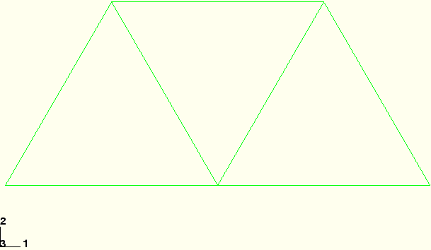
When the job completes successfully, you are ready to view the results of the analysis with the Visualization module. In the Model Tree, click mouse button 3 on the job named Frame and select Results from the menu that appears to enter the Visualization module. ABAQUS/CAE opens the output database created by the job and displays the undeformed model shape, as shown in Figure 2–12.
You can also enter the Visualization module by selecting Visualization from the Module list located under the toolbar. Select FileThe title block at the bottom of the viewport indicates the following:
The description of the model (from the job description).
The name of the output database (from the name of the analysis job).
The product name (ABAQUS/Standard or ABAQUS/Explicit) and version used to generate the output database.
The date the output database was last modified.
Which step is being displayed.
The increment within the step.
The step time.
You can suppress the display of and customize the title block, state block, and view orientation triad by selecting Viewport![]() Viewport Annotation Options from the main menu bar (for example, many of the figures in this manual do not include the title block).
Viewport Annotation Options from the main menu bar (for example, many of the figures in this manual do not include the title block).
The Results Tree
You will use the Results Tree to query the components of the model. The Results Tree allows easy access to the history output contained in an output database file for the purpose of creating X–Y plots and also to groups of elements, nodes, and surfaces based on set names, material and section assignment, etc. for the purposes of verifying the model and also controlling the viewport display.
To query the model:
In the left side of the main window, click the Results tab to switch to the Results Tree if it is not already visible.
All output database files that are open in a given postprocessing session are listed underneath the Output Databases container. Expand this container and then expand the container for the output database named Frame.odb.
Expand the Materials container and click the material named STEEL.
All elements are highlighted in the viewport because only one material assignment was used in this analysis.
The Results Tree will be used more extensively in later examples to illustrate the X–Y plotting capability and manipulating the display using display groups.
Customizing an undeformed shape plot
You will now use the plot options to enable the display of node and element numbering. Plot options that are common to all plot types (undeformed, deformed, contour, symbol, and material orientation) are set in a single dialog box. The contour, symbol, and material orientation plot types have additional options, each specific to the given plot type.
To display node numbers:
From the main menu bar, select Options![]() Common; or use the
Common; or use the ![]() tool in the toolbox.
tool in the toolbox.
The Common Plot Options dialog box appears.
Click the Labels tab.
Toggle on Show node labels.
Click Apply.
ABAQUS/CAE applies the change and keeps the dialog box open.
To display element numbers:
In the Labels tabbed page of the Common Plot Options dialog box, toggle on Show element labels.
Click OK.
ABAQUS/CAE applies the change and closes the dialog box.
Remove the node and element labels before proceeding. To disable the display of node and element numbers, repeat the above procedure and, under Labels, toggle off Show node labels and Show element labels.
Displaying and customizing a deformed shape plot
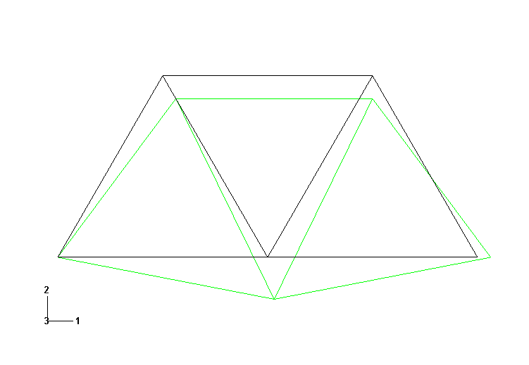
You will now display the deformed model shape and use the plot options to change the deformation scale factor. You will also superimpose the undeformed model shape on the deformed model shape.
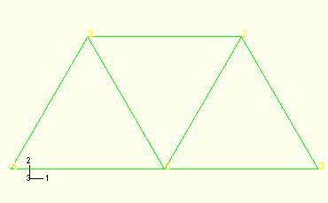
From the main menu bar, select Plot![]() Deformed Shape; or use the
Deformed Shape; or use the ![]() tool in the toolbox. ABAQUS/CAE displays the deformed model shape, as shown in Figure 2–15.
tool in the toolbox. ABAQUS/CAE displays the deformed model shape, as shown in Figure 2–15.
For small-displacement analyses (the default formulation in ABAQUS/Standard) the displacements are scaled automatically to ensure that they are clearly visible. The scale factor is displayed in the state block. In this case the displacements have been scaled by a factor of 42.83.
To change the deformation scale factor:
From the main menu bar, select Options![]() Common; or use the
Common; or use the ![]() tool in the toolbox.
tool in the toolbox.
From the Common Plot Options dialog box, click the Basic tab if it is not already selected.
From the Deformation Scale Factor area, toggle on Uniform and enter 10.0 in the Value field.
Click Apply to redisplay the deformed shape.
The state block displays the new scale factor.
To superimpose the undeformed model shape on the deformed model shape:
Click the ![]() tool in the toolbox to allow multiple plot states in the viewport; then click the
tool in the toolbox to allow multiple plot states in the viewport; then click the ![]() tool or select Plot
tool or select Plot![]() Undeformed Shape to add the undeformed shape plot to the existing deformed plot in the viewport.
Undeformed Shape to add the undeformed shape plot to the existing deformed plot in the viewport.
By default, ABAQUS/CAE plots the deformed model shape in green and the (superimposed) undeformed model shape in a translucent white (appears gray).
The plot options for the superimposed image are controlled separately from those of the primary image. From the main menu bar, select Options![]() Superimpose; or use the
Superimpose; or use the ![]() tool in the toolbox to suppress the translucency of the superimposed (i.e., undeformed) image.
tool in the toolbox to suppress the translucency of the superimposed (i.e., undeformed) image.
From the Superimpose Plot Options dialog box, click the Other tab.
In the Other tabbed page, select the Translucency tab.
Toggle off Apply translucency.
Click OK to close the Superimpose Plot Options dialog box and to apply the changes.
Checking the model with ABAQUS/CAE
You can use ABAQUS/CAE to check that the model is correct before running the simulation. You have already learned how to draw plots of the model and to display the node and element numbers. These are useful tools for checking that ABAQUS is using the correct mesh.
The boundary conditions applied to the overhead hoist model can also be displayed and checked in the Visualization module.
To display boundary conditions on the undeformed model:
Click the ![]() tool in the toolbox to disable multiple plot states in the viewport.
tool in the toolbox to disable multiple plot states in the viewport.
Display the undeformed model shape, if it is not displayed already. From the main menu bar, select Plot![]() Undeformed Shape; or use the
Undeformed Shape; or use the ![]() tool in the toolbox.
tool in the toolbox.
From the main menu bar, select View![]() ODB Display Options.
ODB Display Options.
In the ODB Display Options dialog box, click the Entity Display tab.
Toggle on Show boundary conditions.
Click OK.
ABAQUS/CAE displays symbols to indicate the applied boundary conditions, as shown in Figure 2–17.
Tabular data reports
In addition to the graphical capabilities described above, ABAQUS/CAE allows you to write data to a text file in a tabular format. This feature is a convenient alternative to writing tabular output to the data (.dat) file. Output generated this way has many uses; for example, it can be used in written reports. In this problem you will generate a report containing the element stresses, nodal displacements, and reaction forces.
To generate field data reports:
From the main menu bar, select Report![]() Field Output.
Field Output.
In the Variable tabbed page of the Report Field Output dialog box, accept the default position labeled Integration Point. Click the triangle next to S: Stress components to expand the list of available variables. From this list, toggle on S11.
In the Setup tabbed page, name the report Frame.rpt. In the Data region at the bottom of the page, toggle off Column totals.
Click Apply.
The element stresses are written to the report file.
In the Variable tabbed page of the Report Field Output dialog box, change the position to Unique Nodal. Toggle off S: Stress components, and select U1 and U2 from the list of available U: Spatial displacement variables.
Click Apply.
The nodal displacements are appended to the report file.
In the Variable tabbed page of the Report Field Output dialog box, toggle off U: Spatial displacement, and select RF1 and RF2 from the list of available RF: Reaction force variables.
In the Data region at the bottom of the Setup tabbed page, toggle on Column totals.
Click OK.
The reaction forces are appended to the report file, and the Report Field Output dialog box closes.
Stress output:
Field Output Report

Source 1
---------

   ODB: Frame.odb
   Step: Apply load
   Frame: Increment      1: Step Time =   2.2200E-16

Loc 1 : Integration point values from source 1

Output sorted by column "Element Label".

Field Output reported at integration points for part: FRAME-1
         Element             Int           S.S11
           Label              Pt          @Loc 1
-------------------------------------------------
               1               1    -294.116E+06
               2               1    -294.116E+06
               3               1    -294.116E+06
               4               1     294.116E+06
               5               1     147.058E+06
               6               1     147.058E+06
               7               1     294.116E+06


  Minimum                           -294.116E+06
      At Element                               3

          Int Pt                               1
  Maximum                            294.116E+06
      At Element                               7

          Int Pt                               1
Displacement output:
Field Output Report

Source 1
---------

   ODB: Frame.odb
   Step: Apply load
   Frame: Increment      1: Step Time =   2.2200E-16

Loc 1 : Nodal values from source 1

Output sorted by column "Node Label".

Field Output reported at nodes for part: FRAME-1

            Node            U.U1            U.U2
           Label          @Loc 1          @Loc 1
-------------------------------------------------
               1     1.47058E-03    -2.54712E-03
               2    -46.3235E-12    -2.54712E-03
               3     1.47058E-03         -5.E-33
               4              0.         -5.E-33
               5     735.291E-06    -4.66972E-03


  Minimum           -46.3235E-12    -4.66972E-03

         At Node               2               5
  Maximum            1.47058E-03         -5.E-33

         At Node               3               4
Reaction force output:
Field Output Report

Source 1
---------

   ODB: Frame.odb
   Step: Apply load
   Frame: Increment      1: Step Time =   2.2200E-16

Loc 1 : Nodal values from source 1

Output sorted by column "Node Label".

Field Output reported at nodes for part: FRAME-1

            Node          RF.RF1          RF.RF2
           Label          @Loc 1          @Loc 1
-------------------------------------------------
               1              0.              0.
               2              0.              0.
               3              0.          5.E+03
               4              0.          5.E+03
               5              0.              0.


  Minimum                     0.              0.
         At Node               5               5

  Maximum                     0.          5.E+03
         At Node               5               4

           Total              0.         10.E+03
It is always a good idea to check that the results of the simulation satisfy basic physical principles. In this case check that the external forces applied to the hoist and the reaction forces sum to zero in both the vertical and horizontal directions.
What nodes have vertical forces applied to them? What nodes have horizontal forces? Do the results from your simulation match those shown here?
We will rerun the same analysis in ABAQUS/Explicit for comparison. This time we are interested in the dynamic response of the hoist to the same load applied suddenly at the center. Before continuing, click the Model tab in the left side of the main window to switch to the Model Tree. Click mouse button 3 on Model-1 in the Model Tree and select Copy Model from the menu that appears to copy the existing model to a new model named Explicit. Make all subsequent changes to the Explicit model (you may want to collapse the original model to avoid confusion). You will need to replace the static step with an explicit dynamic step, modify the output requests and the material definition, and change the element library before you can resubmit the job.
Replacing the analysis step
The step definition must change to reflect a dynamic, explicit analysis.
To replace the static step with an explicit dynamic step:
In the Model Tree, expand the Steps container. Click mouse button 3 on the step named Apply load, and select Replace from the menu that appears.
In the Replace Step dialog box, select Dynamic, Explicit from the list of available General procedures. Click Continue.
Model attributes such as boundary conditions, loads, and contact interactions are retained when replacing a step. Model attributes that cannot be converted will be deleted. In this simulation all necessary model attributes will be retained.
In the Basic tabbed page of the Edit Step dialog box, enter the step description 10 kN central load, suddenly applied and set the time period of the step to 0.01 s.
Modifying the output requests
Because this is a dynamic analysis in which the transient response of the frame is of interest, it is helpful to have the displacements of the center point written as history output. Displacement history output can be requested only for a preselected set. Thus, you will create a set that contains the vertex at the center of the bottom of the truss. Then you will add displacements to the history output requests.
To create a set:
In the Model Tree, expand the Assembly container and double-click the Sets item.
The Create Set dialog box appears.
Name the set Center, and click Continue.
In the viewport, select the point at the center of the bottom edge of the truss. In the prompt area, click Done when you are finished.
To add displacements to the history output request:
In the Model Tree, click mouse button 3 on the History Output Requests container and select Manager from the menu that appears.
In the History Output Requests Manager dialog box that appears, click Edit.
The history output editor appears.
Under the Domain field, select Set. ABAQUS automatically provides a list of all the sets created for a given model. In this case you have created only one set, Center.
In the Output Variables region, toggle off the Energy output and click the arrow to the left of the Displacement/Velocity/Acceleration category to reveal history output options for translations and rotations.
Toggle on U, Translations and rotations to have the translations and rotations for the selected set be written as history output to the output database file.
Click OK to save your changes and to close the dialog box. Dismiss the History Output Requests Manager.
Modifying the material definition
Since ABAQUS/Explicit performs a dynamic analysis, a complete material definition requires that you specify the material density. For this problem assume the density is equal to 7800 kg/m3.
To add density to the material definition:
In the Model Tree, expand the Materials container and double-click Steel.
In the material editor, select General![]() Density and type a value of 7800 for the density.
Density and type a value of 7800 for the density.
Click OK to close the Edit Material dialog box.
Changing the element library and submitting the job for analysis
As will be discussed in Chapter 3, “Finite Elements and Rigid Bodies,” the elements available in ABAQUS/Explicit are a subset of those available in ABAQUS/Standard. Thus, to ensure that you are using a valid element type in your analysis, you must change the element library from which the elements are selected to the explicit element library. ABAQUS/CAE automatically filters the available element types according to the selected element library. After changing the element library, you will create and run a new job for the ABAQUS/Explicit analysis.
To change the element library:
In the Model Tree, expand the Frame item underneath the Parts container. Then double-click Mesh in the list that appears.
ABAQUS/CAE switches to the Mesh module.
From the main menu bar, select Mesh![]() Element Type, select the entire frame in the viewport, and change the Element Library selection to Explicit.
Element Type, select the entire frame in the viewport, and change the Element Library selection to Explicit.
Click OK to accept the new element type.
To create and run the new job:
In the Model Tree, double-click the Jobs container.
Name the new job expFrame, and select Explicit as the source model.
Set the Job Type to Full analysis, and submit the job.
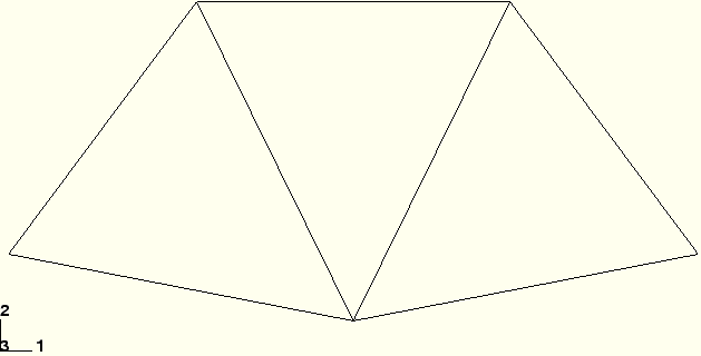
For the static linear perturbation analysis done in ABAQUS/Standard you examined the deformed shape as well as stress, displacement, and reaction force output. For the ABAQUS/Explicit analysis you can similarly examine the deformed shape and generate field data reports. Because this is a dynamic analysis, you should also examine the transient response resulting from the loading. You will do this by animating the time history of the deformed model shape and plotting the displacement history of the bottom center node in the truss.
Plot the deformed shape of the model. For large-displacement analyses (the default formulation in ABAQUS/Explicit) the displaced shape scale factor has a default value of 1. Change the Deformation Scale Factor to 20 so that you can more easily see the deformation of the truss.
To create a time-history animation of the deformed model shape:
From the main menu bar, select Animate![]() Time History; or use the
Time History; or use the ![]() tool in the toolbox.
tool in the toolbox.
The time history animation begins in a continuous loop at its fastest speed. ABAQUS/CAE displays the movie player controls in the right side of the context bar (immediately above the viewport).
From the main menu bar, select Options![]() Animation; or use the animation options
Animation; or use the animation options ![]() tool in the toolbox (located directly underneath the
tool in the toolbox (located directly underneath the ![]() tool).
tool).
The Animation Options dialog box appears.
Change the Mode to Play Once, and slow the animation down by moving the Frame Rate slider.
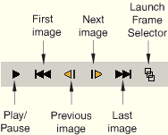
You can use the animation controls to start, pause, and step through the animation. From left to right, these controls perform the following functions: play/pause, first, previous, next, and last.
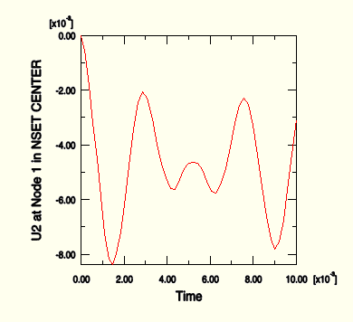
The instantaneous load on the truss causes it to respond dynamically during the 0.01 s of the analysis. You can more closely observe this by plotting the vertical displacement of the node set Center.
You can create X–Y curves from either history or field data stored in the output database (.odb) file. X–Y curves can also be read from an external file or they can be typed into the Visualization module interactively. Once curves have been created, their data can be further manipulated and plotted to the screen in graphical form. In this example you will create and plot the curve using history data.
To create an X–Y plot of the vertical displacement for a node:
In the Results Tree, expand the History Output container underneath the output database named expFrame.odb.
From the list of available history output, double-click Spatial displacement: U2 at Node x in NSET CENTER.
ABAQUS/CAE plots the vertical displacement at the center node along the bottom of the truss, as shown in figure Figure 2–18.
Exiting ABAQUS/CAE
Save your model database file; then select File![]() Exit from the main menu bar to exit ABAQUS/CAE.
Exit from the main menu bar to exit ABAQUS/CAE.