ABAQUS/Standard and ABAQUS/Explicit are capable of solving a wide variety of problems. The characteristics of implicit and explicit procedures determine which method is appropriate for a given problem. For those problems that can be solved with either method, the efficiency with which the problem can be solved can determine which product to use. Understanding the characteristics of implicit and explicit procedures will help you answer this question. Table 2–2 lists the key differences between the analysis products, which are discussed in detail in the relevant chapters in this guide.
Table 2–2 Key differences between ABAQUS/Standard and ABAQUS/Explicit.
| Quantity | ABAQUS/Standard | ABAQUS/Explicit |
|---|---|---|
| Element library | Offers an extensive element library. | Offers an extensive library of elements well suited for explicit analyses. The elements available are a subset of those available in ABAQUS/Standard. |
| Analysis procedures | General and linear perturbation procedures are available. | General procedures are available. |
| Material models | Offers a wide range of material models. | Similar to those available in ABAQUS/Standard; a notable difference is that failure material models are allowed. |
| Contact formulation | Has a robust capability for solving contact problems. | Has a robust contact functionality that readily solves even the most complex contact simulations. |
| Solution technique | Uses a stiffness-based solution technique that is unconditionally stable. | Uses an explicit integration solution technique that is conditionally stable. |
| Disk space and memory | Due to the large numbers of iterations possible in an increment, disk space and memory usage can be large. | Disk space and memory usage is typically much smaller than that for ABAQUS/Standard. |
For many analyses it is clear whether ABAQUS/Standard or ABAQUS/Explicit should be used. For example, as demonstrated in Chapter 8, “Nonlinearity,” ABAQUS/Standard is more efficient for solving smooth nonlinear problems; on the other hand, ABAQUS/Explicit is the clear choice for a wave propagation analysis. There are, however, certain static or quasi-static problems that can be simulated well with either program. Typically, these are problems that usually would be solved with ABAQUS/Standard but may have difficulty converging because of contact or material complexities, resulting in a large number of iterations. Such analyses are expensive in ABAQUS/Standard because each iteration requires a large set of linear equations to be solved.
Whereas ABAQUS/Standard must iterate to determine the solution to a nonlinear problem, ABAQUS/Explicit determines the solution without iterating by explicitly advancing the kinematic state from the previous increment. Even though a given analysis may require a large number of time increments using the explicit method, the analysis can be more efficient in ABAQUS/Explicit if the same analysis in ABAQUS/Standard requires many iterations.
Another advantage of ABAQUS/Explicit is that it requires much less disk space and memory than ABAQUS/Standard for the same simulation. For problems in which the computational cost of the two programs may be comparable, the substantial disk space and memory savings of ABAQUS/Explicit make it attractive.
Using the explicit method, the computational cost is proportional to the number of elements and roughly inversely proportional to the smallest element dimension. Mesh refinement, therefore, increases the computational cost by increasing the number of elements and reducing the smallest element dimension. As an example, consider a three-dimensional model with uniform, square elements. If the mesh is refined by a factor of two in all three directions, the computational cost increases by a factor of 2 × 2 × 2 as a result of the increase in the number of elements and by a factor of 2 as a result of the decrease in the smallest element dimension. The total computational cost of the analysis increases by a factor of 24, or 16, by refining the mesh. Disk space and memory requirements are proportional to the number of elements with no dependence on element dimensions; thus, these requirements increase by a factor of 8.
Whereas predicting the cost increase with mesh refinement for the explicit method is rather straightforward, cost is more difficult to predict when using the implicit method. The difficulty arises from the problem-dependent relationship between element connectivity and solution cost, a relationship that does not exist in the explicit method. Using the implicit method, experience shows that for many problems the computational cost is roughly proportional to the square of the number of degrees of freedom. Consider the same example of a three-dimensional model with uniform, square elements. Refining the mesh by a factor of two in all three directions increases the number of degrees of freedom by approximately 23, causing the computational cost to increase by a factor of roughly (23)2, or 64. The disk space and memory requirements increase in the same manner, although the actual increase is difficult to predict.
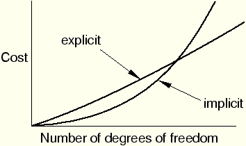
The explicit method shows great cost savings over the implicit method as the model size increases, as long as the mesh is relatively uniform. Figure 2–19 illustrates the comparison of cost versus model size using the explicit and implicit methods. For this problem the number of degrees of freedom scales with the number of elements.