Product: ABAQUS/Standard
The inelastic constitutive theory provided in ABAQUS/Standard for modeling cohesionless materials is based on the critical state plasticity theory developed by Roscoe and his colleagues at Cambridge (Schofield et al., 1968, and Parry, 1972). The specific model implemented is an extension of the “modified Cam-clay” theory. The discussion is entirely in terms of effective stress: the soil may be saturated with a permeating fluid that carries a pressure stress and is assumed to flow according to Darcy's law. The continuum theory of this two phase material is described in “Continuity statement for the wetting liquid phase in a porous medium,” Section 2.8.4.
The modified Cam-clay theory is a classical plasticity model. It uses a strain rate decomposition in which the rate of mechanical deformation of the soil is decomposed into an elastic and a plastic part; an elasticity theory; a yield surface; a flow rule; and a hardening rule. These various parts of the theory are defined in this section. The model is implemented numerically using backward Euler integration of the flow rule and hardening rule: this approach is used throughout ABAQUS for plasticity models.
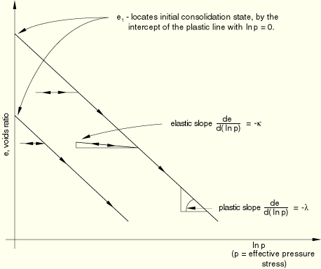
The basic ideas of the Cam-clay model are shown geometrically in Figure 4.4.3–1 to Figure 4.4.3–7. The main features of the model are the use of an elastic model (either linear elasticity or the porous elasticity model, which exhibits an increasing bulk elastic stiffness as the material undergoes compression) and for the inelastic part of the deformation a particular form of yield surface with associated flow and a hardening rule that allows the yield surface to grow or shrink.
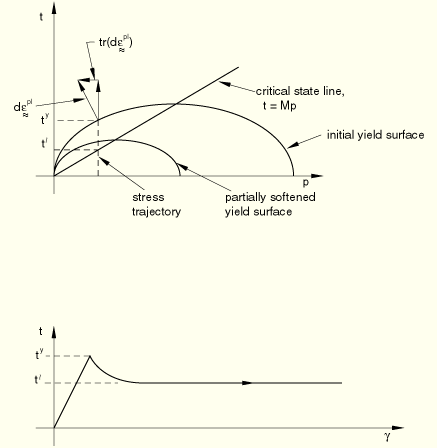
A key feature of the model is the hardening/softening concept, which is developed around the introduction of a “critical state” surface: the locus of effective stress states where unrestricted, purely deviatoric, plastic flow of the soil skeleton occurs under constant effective stress. This critical state surface is assumed to be a cone in the space of principal effective stress (Figure 4.4.3–1), whose vertex is the origin (zero effective stress) and whose axis is the equivalent pressure stress, ![]() .
.
The hardening/softening assumption controls the size of the yield surface in effective stress space. The hardening/softening is assumed to depend only on the volumetric plastic strain component and is such that, when the volumetric plastic strain is compressive (that is, when the soil skeleton is compacted), the yield surface grows in size, while inelastic increase in the volume of the soil skeleton causes the yield surface to shrink. The choice of elliptical arcs for the yield surface in the (![]() ) plane, together with the associated flow assumption, thus causes softening of the material for yielding states where
) plane, together with the associated flow assumption, thus causes softening of the material for yielding states where ![]() (to the left of the critical state line in Figure 4.4.3–2, the “dry” side of critical state) and hardening of the material for yielding states where
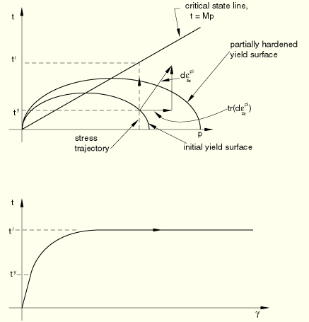
(to the left of the critical state line in Figure 4.4.3–2, the “dry” side of critical state) and hardening of the material for yielding states where ![]() (to the right of the critical state line in Figure 4.4.3–3, the “wet” side of critical state).
(to the right of the critical state line in Figure 4.4.3–3, the “wet” side of critical state).
The preceding discussion describes the concepts of the theory. These are now formalized, as they are implemented in ABAQUS/Standard.
The volume change is decomposed as
whereVolumetric strains are defined as

These definitions and Equation 4.4.3–1 result in the usual additive strain rate decomposition for volumetric strain rates:
The model also assumes the deviatoric strain rates decompose in an additive manner, so that the total strain rates decompose as
![]()
The elastic behavior can be modeled as linear or by using the porous elasticity model, typically with a zero tensile strength, as described in “Porous elasticity,” Section 4.4.1.
The modified Cam-clay yield function is defined in terms of the equivalent effective pressure stress, ![]() , and the Mises equivalent stress and third stress invariant, defined as
, and the Mises equivalent stress and third stress invariant, defined as
The surface is
In this equation ![]() is a user-specified constant that can be a function of temperature
is a user-specified constant that can be a function of temperature ![]() and other predefined field variables
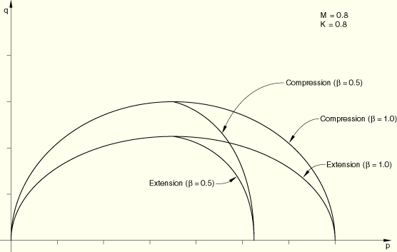
and other predefined field variables ![]() . This constant is used to modify the shape of the yield surface on the “wet” side of critical state, so the elliptic arc on the “wet” side of critical state has a different curvature from the elliptic arc used on the “dry” side:
. This constant is used to modify the shape of the yield surface on the “wet” side of critical state, so the elliptic arc on the “wet” side of critical state has a different curvature from the elliptic arc used on the “dry” side: ![]() on the “dry” side of critical state, while
on the “dry” side of critical state, while ![]() in most cases on the “wet” side, as shown in Figure 4.4.3–4.
in most cases on the “wet” side, as shown in Figure 4.4.3–4. ![]() defines the hardening of the plasticity model, and is the point on the
defines the hardening of the plasticity model, and is the point on the ![]() -axis at which the elliptic arcs of the yield surface intersect the critical state line, as indicated in Figure 4.4.3–4.
-axis at which the elliptic arcs of the yield surface intersect the critical state line, as indicated in Figure 4.4.3–4. ![]() is the slope of the critical state line in the
is the slope of the critical state line in the ![]() –
–![]() plane (the ratio of
plane (the ratio of ![]() to
to ![]() at critical state); and
at critical state); and ![]() , where
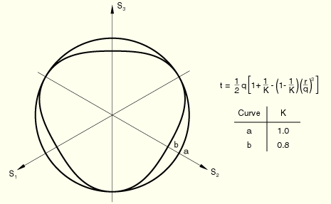
, where ![]() is used to shape the yield surface in the
is used to shape the yield surface in the ![]() plane, and is defined as
plane, and is defined as
![]()
Associated flow is used with the modified Cam-clay plasticity model. The size of the yield surface is defined by ![]() : the evolution of this variable, therefore, characterizes the hardening or softening of the material. It is observed experimentally that, during plastic deformation,
: the evolution of this variable, therefore, characterizes the hardening or softening of the material. It is observed experimentally that, during plastic deformation,
![]()
![]()
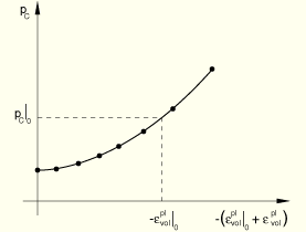
The evolution of the yield surface can alternatively be defined as a piecewise linear function relating the yield stress in hydrostatic compression, ![]() , and the corresponding volumetric plastic strain
, and the corresponding volumetric plastic strain ![]() (Figure 4.4.3–7):
(Figure 4.4.3–7):
![]()
![]()
ABAQUS checks that the initial effective stress state lies inside or on the initial yield surface. At any material point where the yield function is violated, ![]() is adjusted so that Equation 4.4.3–3 is satisfied exactly (and, hence, the initial stress state lies on the yield surface).
is adjusted so that Equation 4.4.3–3 is satisfied exactly (and, hence, the initial stress state lies on the yield surface).