Products: ABAQUS/Standard ABAQUS/Explicit
The behavior of granular and polymeric materials is complex. However, under essentially monotonic loading conditions rather simple constitutive models provide useful design information. These constitutive models are essentially pressure-dependent plasticity models that have historically been popular in the geotechnical engineering field. However, more recently they have also been found to be useful for the modeling of some polymeric and composite materials that exhibit significantly different yield behavior in tension and compression.
The models described here are extensions of the original Drucker-Prager model (Drucker and Prager, 1952). In the context of geotechnical materials the extensions of interest include the use of curved yield surfaces in the meridional plane, the use of noncircular yield surfaces in the deviatoric stress plane, and the use of nonassociated flow laws. In the context of polymeric and composite materials, the extensions of interest are mainly the use of nonassociated flow laws and the inclusion of rate-dependent effects. In both contexts the models have been extended to include creep.
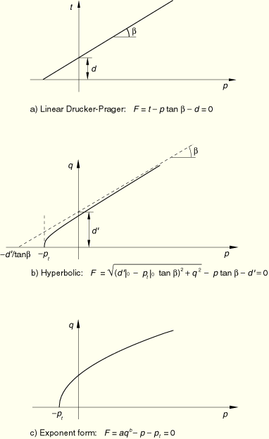
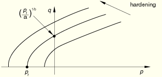
Three yield criteria are provided in this set of models. They offer differently shaped yield surfaces in the meridional plane (![]() –
–![]() plane): a linear form, a hyperbolic form, and a general exponent form (see Figure 4.4.2–1).
plane): a linear form, a hyperbolic form, and a general exponent form (see Figure 4.4.2–1).
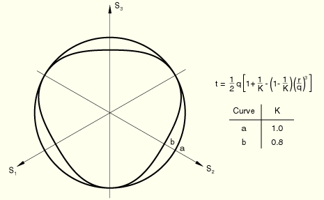
The linear model (available in ABAQUS/Standard and ABAQUS/Explicit) provides a noncircular section in the deviatoric (![]() ) plane, associated inelastic flow in the deviatoric plane, and separate dilation and friction angles. The smoothed surface used in the deviatoric plane differs from a true Mohr-Coulomb surface that exhibits vertices. This has restrictive implications, especially with respect to flow localization studies for granular materials, but this may not be of major significance in many routine design applications. Input data parameters define the shape of the yield and flow surfaces in the deviatoric plane as well as the friction and dilation angles, so that a range of simple theories is provided; for example, the original Drucker-Prager model (Drucker and Prager, 1952) is available within this model.
) plane, associated inelastic flow in the deviatoric plane, and separate dilation and friction angles. The smoothed surface used in the deviatoric plane differs from a true Mohr-Coulomb surface that exhibits vertices. This has restrictive implications, especially with respect to flow localization studies for granular materials, but this may not be of major significance in many routine design applications. Input data parameters define the shape of the yield and flow surfaces in the deviatoric plane as well as the friction and dilation angles, so that a range of simple theories is provided; for example, the original Drucker-Prager model (Drucker and Prager, 1952) is available within this model.
The hyperbolic and general exponent models (available in ABAQUS/Standard only) use a von Mises (circular) section in the deviatoric stress plane with associated plastic flow. A hyperbolic flow potential is used in the meridional plane, which—in general—means nonassociated flow.
Perfect plasticity as well as isotropic hardening are offered with these models. Isotropic hardening is generally considered to be a suitable model for problems in which the plastic straining goes well beyond the incipient yield state where the Bauschinger effect is noticeable (Rice, 1975). This hardening theory is, therefore, used for processes involving large plastic strain and in which the plastic strain rate does not continuously reverse direction sharply; that is, the models are intended for problems involving essentially monotonic loading, as distinct from cyclic loading.
The isotropic hardening models can be used for rate-dependent as well as rate-independent behavior. The rate-dependent version is intended for relatively high strain rate applications.
Isotropic hardening means that the yield function is written as
![]()
The equivalent plastic strain rate, ![]() , is defined for the linear Drucker-Prager model as
, is defined for the linear Drucker-Prager model as
The functional dependence ![]() can include hardening as well as rate-dependent effects. If the shapes of the stress-strain curves are different at different strain rates, the test data are entered as tables of yield stress values versus equivalent plastic strain at different equivalent plastic strain rates: one table per strain rate. The yield stress at a given strain and strain rate is interpolated directly from these tables.
can include hardening as well as rate-dependent effects. If the shapes of the stress-strain curves are different at different strain rates, the test data are entered as tables of yield stress values versus equivalent plastic strain at different equivalent plastic strain rates: one table per strain rate. The yield stress at a given strain and strain rate is interpolated directly from these tables.
Alternatively, when it can be assumed that the shapes of the hardening curves at different strain rates are similar, the hardening and rate dependence are specified separately. In this case we assume that the rate dependence can be written in a separable form:
![]()
Creep models are most suitable for applications that exhibit time-dependent inelastic deformation at low deformation rates. Such inelastic deformation, which can coexist with rate-independent plastic deformation, is described later in this section. However, the existence of creep in an ABAQUS material definition precludes the use of rate dependence as described above.
An additive strain rate decomposition is assumed:
whereThe elastic behavior can be modeled as linear or with the porous elasticity model including tensile strength described in “Porous elasticity,” Section 4.4.1. If creep has been defined, the elastic behavior must be modeled as linear.
In this model we define a deviatoric stress measure
With this expression for the deviatoric stress measure, the yield surface is defined as
where
In the case of hardening defined in uniaxial compression, the linear yield criterion precludes friction angles ![]() 71.5° (
71.5° (![]() 3). This is not seen as a limitation since it is unlikely this will be the case for real materials.
3). This is not seen as a limitation since it is unlikely this will be the case for real materials.
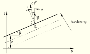
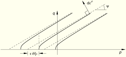
The hardening parameter ![]() measures the cohesion of the material and represents isotropic hardening, as illustrated in Figure 4.4.2–3.
measures the cohesion of the material and represents isotropic hardening, as illustrated in Figure 4.4.2–3.
A method for converting Mohr-Coulomb data (![]() , the angle of Coulomb friction, and
, the angle of Coulomb friction, and ![]() , the cohesion) to appropriate values of
, the cohesion) to appropriate values of ![]() and
and ![]() is described in the ABAQUS Analysis User's Manual.
is described in the ABAQUS Analysis User's Manual.
Potential flow in the linear model is assumed, so that
where
Comparison of Equation 4.4.2–3 and Equation 4.4.2–5 shows that the flow is associated in the deviatoric plane, because the yield surface and the flow potential both have the same functional dependence on ![]() . However, the dilation angle,
. However, the dilation angle, ![]() , and the material friction angle,
, and the material friction angle, ![]() , may be different, so the model may not be associated in the
, may be different, so the model may not be associated in the ![]() –
–![]() plane. For
plane. For ![]() the material is nondilational; and if
the material is nondilational; and if ![]() , the model is fully associated—the model is then of the type first introduced by Drucker and Prager (1952). For
, the model is fully associated—the model is then of the type first introduced by Drucker and Prager (1952). For ![]() and
and ![]() the original Drucker-Prager model is recovered.
the original Drucker-Prager model is recovered.
The hyperbolic and general exponent models, which are only available in ABAQUS/Standard, are written in terms of the first two stress invariants only. The hyperbolic yield criterion is a continuous combination of the maximum tensile stress condition of Rankine (tensile cut-off) and the linear Drucker-Prager condition at high confining stress. It is written as
where
The general exponent form provides the most general yield criterion available in this class of models. The yield function is written as
where
The material parameters ![]() ,
, ![]() , and
, and ![]() can be given directly; or, if triaxial test data at different levels of confining pressure are available, ABAQUS will determine the material parameters from the triaxial test data. A least squares fit, which minimizes the relative error in stress, is used to obtain the “best fit” values for
can be given directly; or, if triaxial test data at different levels of confining pressure are available, ABAQUS will determine the material parameters from the triaxial test data. A least squares fit, which minimizes the relative error in stress, is used to obtain the “best fit” values for ![]() ,
, ![]() , and
, and ![]() .
.
Potential flow in the hyperbolic and general exponent models is assumed, so that
where![]()

In both models flow is associated in the deviatoric stress plane. In the general exponent model, flow is always nonassociated in the meridional ![]() –
–![]() plane. In the hyperbolic model comparison of Equation 4.4.2–6 and Equation 4.4.2–9 shows that the flow is nonassociated in the
plane. In the hyperbolic model comparison of Equation 4.4.2–6 and Equation 4.4.2–9 shows that the flow is nonassociated in the ![]() –
–![]() plane if the dilation angle,
plane if the dilation angle, ![]() , and the material friction angle,
, and the material friction angle, ![]() , are different. The hyperbolic model provides associated flow in the
, are different. The hyperbolic model provides associated flow in the ![]() –
–![]() plane only when
plane only when ![]() and
and ![]() .
.
Classical “creep” behavior of materials that exhibit plastic behavior according to the extended Drucker-Prager models can be defined.
The creep behavior in such materials is intimately tied to the plasticity behavior (through the definition of the creep flow potential and test data), so it is necessary to define the Drucker-Prager plasticity and hardening behavior as well. The elastic part of the behavior must be linear.
The rate-independent part of the plastic behavior is limited to the linear Drucker-Prager model with a von Mises (circular) section in the deviatoric stress plane (![]() =1). The plastic potential is the hyperbolic flow potential described in conjunction with the hyperbolic and general exponent models (Equation 4.4.2–9).
=1). The plastic potential is the hyperbolic flow potential described in conjunction with the hyperbolic and general exponent models (Equation 4.4.2–9).
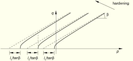
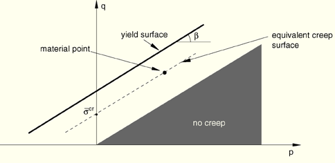
We adopt the notion of creep isosurfaces (or equivalent creep surfaces) of stress points that share the same creep “intensity,” as measured by an equivalent creep stress. When the material plastifies, the equivalent creep surface should coincide with the yield surface; therefore, we define the equivalent creep surfaces by homogeneously scaling down the yield surface. In the ![]() –
–![]() plane that translates into parallels to the yield surface, as depicted in Figure 4.4.2–7.
plane that translates into parallels to the yield surface, as depicted in Figure 4.4.2–7.
Figure 4.4.2–7 shows how the equivalent creep stress is determined when the material properties are defined via a shear test: a parallel to the yield surface is drawn, such that it passes by the material point; the intersection of such a line with the test stress path (![]() ) produces
) produces ![]() .
.
This approach has the consequence that the creep strain rate is a function of both ![]() and
and ![]() and allows realistic material properties to be determined in cases in which, due to high hydrostatic pressures,
and allows realistic material properties to be determined in cases in which, due to high hydrostatic pressures, ![]() is very high. If one looks at the yield strength of this material to be a composite of cohesion strength and friction strength, this model corresponds to cohesion-determined creep. Thus, there is a cone in
is very high. If one looks at the yield strength of this material to be a composite of cohesion strength and friction strength, this model corresponds to cohesion-determined creep. Thus, there is a cone in ![]() –
–![]() space inside which there is no creep.
space inside which there is no creep.
The built-in ABAQUS creep laws or the uniaxial laws defined through user subroutine CREEP can be used. The integration of the creep strain rate is first attempted explicitly, as described in “Rate-dependent metal plasticity (creep),” Section 4.3.4. If the stability limit is exceeded, a geometrically nonlinear analysis is being performed, or plasticity becomes active, the integration is done by the backward Euler method, as described in “Rate-dependent metal plasticity (creep),” Section 4.3.4.
The creep flow rule is derived from a creep potential, ![]() , in such a way that
, in such a way that
![]()
![]()
The creep strain rate is assumed to follow from the same hyperbolic potential as the plastic strain rate
whereEquation 4.4.2–10 and Equation 4.4.2–11 produce the complete flow rule
where![]()
![]()
![]()
![]()
An example of “slow” loading in which the approximation is visible is included in “Verification of creep integration,” Section 3.2.6 of the ABAQUS Benchmarks Manual. As is clear in the example, the effect of the approximation is small in spite of the fact that the load is ramped up over the step.
Although creep flow is associated in the deviatoric stress plane, the use of a creep potential different from the equivalent creep surface implies that creep flow is nonassociated.