Products: ABAQUS/Standard ABAQUS/Explicit
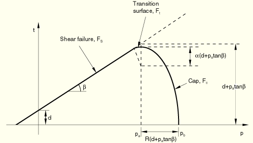
The modified Drucker-Prager/Cap plasticity model in ABAQUS is intended for geological materials that exhibit pressure-dependent yield. The yield surface includes two main segments: a shear failure surface, providing dominantly shearing flow, and a “cap,” which intersects the equivalent pressure stress axis (Figure 4.4.4–1).
There is a transition region between these segments, introduced to provide a smooth surface. The cap serves two main purposes: it bounds the yield surface in hydrostatic compression, thus providing an inelastic hardening mechanism to represent plastic compaction, and it helps to control volume dilatancy when the material yields in shear by providing softening as a function of the inelastic volume increase created as the material yields on the Drucker-Prager shear failure and transition yield surfaces.The model uses associated flow in the cap region and nonassociated flow in the shear failure and transition regions. The model has been extended to include creep, with certain limitations that are outlined in this section. The creep behavior is envisaged as arising out of two possible mechanisms: one dominated by shear behavior and the other dominated by hydrostatic compression.
A linear strain rate decomposition is assumed, so
![]()
The elastic behavior can be modeled as linear elastic or by using the porous elasticity model including tensile strength, described in “Porous elasticity,” Section 4.4.1. If creep has been defined, the elastic behavior must be modeled as linear.
The yield/failure surfaces used with this model are written in terms of the three stress invariants: the equivalent pressure stress,
![]()
![]()
![]()
![]()
We also define the deviatoric stress measure
With this expression for the deviatoric stress measure, the Drucker-Prager failure surface is written as
![]()
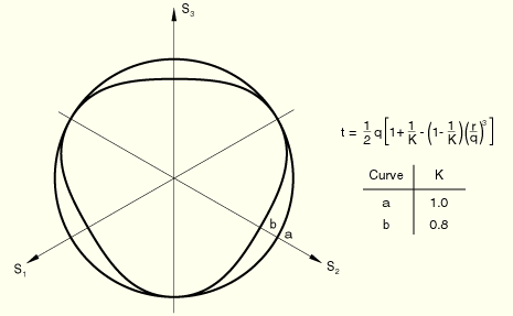
The cap yield surface has an elliptical shape with constant eccentricity in the meridional (![]() –
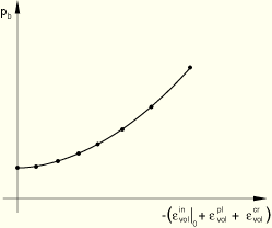
–![]() ) plane (Figure 4.4.4–1) and also includes dependence on the third stress invariant in the deviatoric plane (Figure 4.4.2–2). The cap surface hardens or softens as a function of the volumetric plastic strain: volumetric plastic compaction (when yielding on the cap) causes hardening, while volumetric plastic dilation (when yielding on the shear failure surface) causes softening. The cap yield surface is written as
) plane (Figure 4.4.4–1) and also includes dependence on the third stress invariant in the deviatoric plane (Figure 4.4.2–2). The cap surface hardens or softens as a function of the volumetric plastic strain: volumetric plastic compaction (when yielding on the cap) causes hardening, while volumetric plastic dilation (when yielding on the shear failure surface) causes softening. The cap yield surface is written as
The evolution parameter, ![]() , is defined as
, is defined as
![]()
The parameter ![]() is a small number (typically 0.01 to 0.05) used to define a smooth transition surface between the shear failure surface and the cap:
is a small number (typically 0.01 to 0.05) used to define a smooth transition surface between the shear failure surface and the cap:

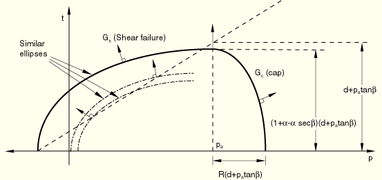
Plastic flow is defined by a flow potential that is associated on the cap and nonassociated on the failure yield surface and transition yield surfaces. The nonassociated nature of these surfaces stems from the shape of the flow potential in the meridional plane. The flow potential surface in the meridional plane is shown in Figure 4.4.4–4.
It is made up of an elliptical portion in the cap region that is identical to the cap yield surface:
Nonassociated flow implies that the material stiffness matrix is not symmetric, so the unsymmetric solver should be invoked by the user. However, if the region of the model in which nonassociated inelastic deformation is occurring is confined, it is possible that a symmetric approximation to the material stiffness matrix will give an acceptable convergence rate: in such cases the unsymmetric solver may not be needed.
Classical “creep” behavior of materials that also exhibit plastic behavior according to the modified Drucker-Prager/Cap model can be defined.
The creep behavior in such materials is intimately tied to the plasticity behavior (through the definition of creep flow potentials and test data), so it is necessary to define the modified Drucker-Prager/Cap plasticity and hardening behavior as well. The elastic part of the behavior must be linear.
The rate-independent part of the plastic behavior is limited by the following restrictions:
![]() —that is, no transition zone is allowed;
—that is, no transition zone is allowed;
K=1—that is, no third stress invariant effects are taken into account.
The built-in ABAQUS creep laws or uniaxial laws defined through user subroutine CREEP can be used. The integration of the creep strain rate is first attempted explicitly, as described in “Rate-dependent metal plasticity (creep),” Section 4.3.4. The integration is done by the backward Euler method (as described in “Rate-dependent metal plasticity (creep),” Section 4.3.4) if the stability limit is exceeded, a geometrically nonlinear analysis is being performed, or plasticity becomes active.
In this model we assume the existence of two separate and independent creep mechanisms. One is a cohesion mechanism, which operates similarly to the Drucker-Prager creep model described in “Models for granular or polymer behavior,” Section 4.4.2. The other is a consolidation mechanism, which operates similarly to the cap zone plasticity. We then have
![]()
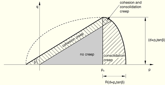
As described above, the cap surface hardens or softens as a function of the volumetric plastic strain and volumetric creep strain: volumetric inelastic compaction (when yielding on the cap or creeping through the consolidation mechanism) causes hardening, while volumetric plastic dilation (when yielding on the shear failure surface or creeping through the cohesion mechanism) causes softening. The separation between the two yield surfaces and the dominant regions for the two creep mechanisms are defined by the evolution parameter, ![]() , which relates to the user-defined hydrostatic compression yield stress,
, which relates to the user-defined hydrostatic compression yield stress, ![]() (Figure 4.4.4–3).
(Figure 4.4.4–3).
The cohesion mechanism is active for all stress states that have a positive equivalent creep stress as explained below. The consolidation mechanism is active for all stress states in which the pressure is larger than ![]() . Figure 4.4.4–5 illustrates the active regions in this formulation.
. Figure 4.4.4–5 illustrates the active regions in this formulation.
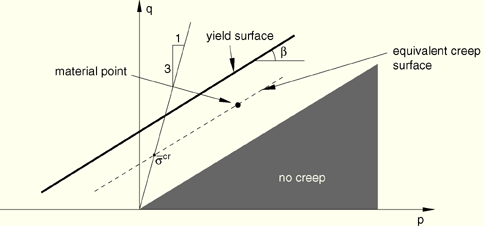
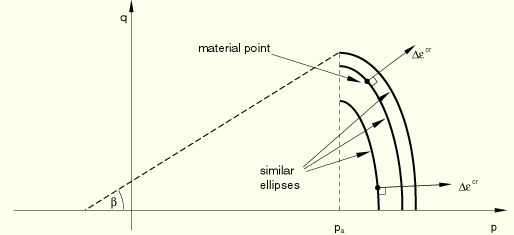
We adopt the notion of the existence of creep isosurfaces (or equivalent creep surfaces) of stress points that share the same creep “intensity,” as measured by an equivalent creep stress. Consider the cohesion creep mechanism first. When the material plastifies, the equivalent creep surface should coincide with the yield surface; therefore, we define the equivalent creep surfaces by homogeneously scaling down the yield surface. In the ![]() –
–![]() plane that translates into parallels to the yield surface, as depicted in Figure 4.4.4–6. ABAQUS requires that cohesion creep properties be measured in a uniaxial compression test.
plane that translates into parallels to the yield surface, as depicted in Figure 4.4.4–6. ABAQUS requires that cohesion creep properties be measured in a uniaxial compression test.
Next consider the consolidation creep mechanism. In this case we wish to make creep dependent on the hydrostatic pressure above a threshold value of ![]() , with a smooth transition to the areas in which the mechanism is not active (
, with a smooth transition to the areas in which the mechanism is not active (![]() ). Therefore, we define equivalent creep surfaces as constant pressure surfaces. In the
). Therefore, we define equivalent creep surfaces as constant pressure surfaces. In the ![]() –
–![]() plane that translates into vertical lines. ABAQUS requires that consolidation creep properties be measured in a hydrostatic compression test. The effective creep pressure,
plane that translates into vertical lines. ABAQUS requires that consolidation creep properties be measured in a hydrostatic compression test. The effective creep pressure, ![]() , is then the point on the
, is then the point on the ![]() -axis with a relative pressure
-axis with a relative pressure
The creep flow rules are derived from creep potentials, ![]() , in such a way that
, in such a way that
![]()
![]()
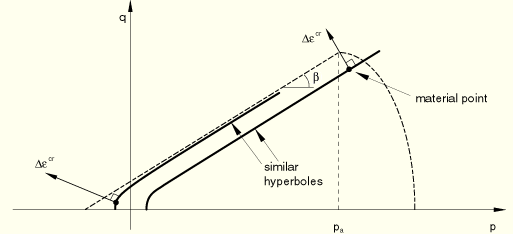
For the cohesion mechanism the creep potential is assumed to follow the same potential as the creep strain rate in the Drucker-Prager creep model (“Models for granular or polymer behavior,” Section 4.4.2); that is, a hyperbolic function. This creep flow potential, which is continuous and smooth, ensures that the flow direction is always uniquely defined. The function approaches a parallel to the shear-failure yield surface asymptotically at high confining pressure stress and intersects the hydrostatic pressure axis at a right angle. A family of hyperbolic potentials in the meridional stress plane is shown in Figure 4.4.4–7:
whereThe equivalent cohesion creep strain rate is then determined from the uniaxial law:
![]()
![]()
![]()
An example of “slow” loading in which the approximation is visible is included in “Verification of creep integration,” Section 3.2.6 of the ABAQUS Benchmarks Manual. As is clear in the example, the effect of the approximation is small in spite of the fact that the load is ramped up over the step.
The equivalent cohesion creep strain rate is a function of both ![]() and
and ![]() through
through ![]() . The creep potential is the von Mises circle in the deviatoric stress plane (the
. The creep potential is the von Mises circle in the deviatoric stress plane (the ![]() -plane). Although creep flow is associated in the deviatoric stress plane, the use of a creep potential different from the equivalent creep surface implies that creep flow is nonassociated.
-plane). Although creep flow is associated in the deviatoric stress plane, the use of a creep potential different from the equivalent creep surface implies that creep flow is nonassociated.
For the consolidation mechanism the creep potential is derived from the plastic potential of the cap zone (Figure 4.4.4–8):
Recall that this mechanism is active only ifThe equivalent consolidation creep strain rate is then determined from the uniaxial law
![]()
Equation 4.4.4–3 and Equation 4.4.4–4 produce ![]() ; and Equation 4.4.4–2, Equation 4.4.4–3, and Equation 4.4.4–6 produce the flow rule for this mechanism:
; and Equation 4.4.4–2, Equation 4.4.4–3, and Equation 4.4.4–6 produce the flow rule for this mechanism:
![]()
![]()
The creep potential is the von Mises circle in the deviatoric stress plane (the ![]() -plane). Creep flow is nonassociated in this mechanism.
-plane). Creep flow is nonassociated in this mechanism.
This formulation is quite simplistic and ignores the effects of ![]() on the creep function,
on the creep function, ![]() . The two creep mechanisms operate independently from each other. This implies that
. The two creep mechanisms operate independently from each other. This implies that ![]() does not depend on
does not depend on ![]() and that
and that ![]() does not depend on
does not depend on ![]() . The only cross effects between both mechanisms are obtained through the dependency of
. The only cross effects between both mechanisms are obtained through the dependency of ![]() on the volumetric creep from any of them.
on the volumetric creep from any of them.