Products: ABAQUS/Standard ABAQUS/Explicit ABAQUS/CAE
The concrete damaged plasticity model in ABAQUS:
provides a general capability for modeling concrete and other quasi-brittle materials in all types of structures (beams, trusses, shells, and solids);
uses concepts of isotropic damaged elasticity in combination with isotropic tensile and compressive plasticity to represent the inelastic behavior of concrete;
can be used for plain concrete, even though it is intended primarily for the analysis of reinforced concrete structures;
can be used with rebar to model concrete reinforcement;
is designed for applications in which concrete is subjected to monotonic, cyclic, and/or dynamic loading under low confining pressures;
consists of the combination of nonassociated multi-hardening plasticity and scalar (isotropic) damaged elasticity to describe the irreversible damage that occurs during the fracturing process;
allows user control of stiffness recovery effects during cyclic load reversals;
can be defined to be sensitive to the rate of straining;
can be used in conjunction with a viscoplastic regularization of the constitutive equations in ABAQUS/Standard to improve the convergence rate in the softening regime;
requires that the elastic behavior of the material be isotropic and linear (see “Defining isotropic elasticity” in “Linear elastic behavior,” Section 17.2.1); and
is defined in detail in “Damaged plasticity model for concrete and other quasi-brittle materials,” Section 4.5.2 of the ABAQUS Theory Manual.
The model is a continuum, plasticity-based, damage model for concrete. It assumes that the main two failure mechanisms are tensile cracking and compressive crushing of the concrete material. The evolution of the yield (or failure) surface is controlled by two hardening variables, ![]() and
and ![]() , linked to failure mechanisms under tension and compression loading, respectively. We refer to
, linked to failure mechanisms under tension and compression loading, respectively. We refer to ![]() and
and ![]() as tensile and compressive equivalent plastic strains, respectively. The following sections discuss the main assumptions about the mechanical behavior of concrete.
as tensile and compressive equivalent plastic strains, respectively. The following sections discuss the main assumptions about the mechanical behavior of concrete.
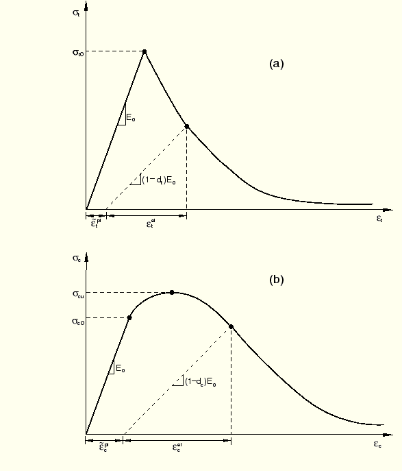
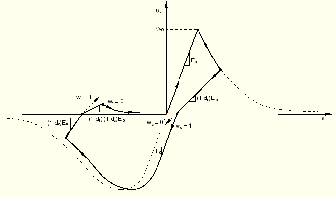
The model assumes that the uniaxial tensile and compressive response of concrete is characterized by damaged plasticity, as shown in Figure 18.5.3–1.
Under uniaxial tension the stress-strain response follows a linear elastic relationship until the value of the failure stress,It is assumed that the uniaxial stress-strain curves can be converted into stress versus plastic-strain curves. (This conversion is performed automatically by ABAQUS from the user-provided stress versus “inelastic” strain data, as explained below.) Thus,
As shown in Figure 18.5.3–1, when the concrete specimen is unloaded from any point on the strain softening branch of the stress-strain curves, the unloading response is weakened: the elastic stiffness of the material appears to be damaged (or degraded). The degradation of the elastic stiffness is characterized by two damage variables, ![]() and
and ![]() , which are assumed to be functions of the plastic strains, temperature, and field variables:
, which are assumed to be functions of the plastic strains, temperature, and field variables:
![]()
If ![]() is the initial (undamaged) elastic stiffness of the material, the stress-strain relations under uniaxial tension and compression loading are, respectively:
is the initial (undamaged) elastic stiffness of the material, the stress-strain relations under uniaxial tension and compression loading are, respectively:
![]()
Under uniaxial cyclic loading conditions the degradation mechanisms are quite complex, involving the opening and closing of previously formed micro-cracks, as well as their interaction. Experimentally, it is observed that there is some recovery of the elastic stiffness as the load changes sign during a uniaxial cyclic test. The stiffness recovery effect, also known as the “unilateral effect,” is an important aspect of the concrete behavior under cyclic loading. The effect is usually more pronounced as the load changes from tension to compression, causing tensile cracks to close, which results in the recovery of the compressive stiffness.
The concrete damaged plasticity model assumes that the reduction of the elastic modulus is given in terms of a scalar degradation variable d as
![]()
This expression holds both in the tensile (![]() ) and the compressive (
) and the compressive (![]() ) sides of the cycle. The stiffness degradation variable, d, is a function of the stress state and the uniaxial damage variables,
) sides of the cycle. The stiffness degradation variable, d, is a function of the stress state and the uniaxial damage variables, ![]() and
and ![]() . For the uniaxial cyclic conditions ABAQUS assumes that
. For the uniaxial cyclic conditions ABAQUS assumes that
![]()
![]()
![]()
![]()
In tension (![]() ),
), ![]() ; therefore,
; therefore, ![]() as expected.
as expected.
In compression (![]() ),
), ![]() , and
, and ![]() . If
. If ![]() , then
, then ![]() ; therefore, the material fully recovers the compressive stiffness (which in this case is the initial undamaged stiffness,
; therefore, the material fully recovers the compressive stiffness (which in this case is the initial undamaged stiffness, ![]() ). If, on the other hand,
). If, on the other hand, ![]() , then
, then ![]() and there is no stiffness recovery. Intermediate values of
and there is no stiffness recovery. Intermediate values of ![]() result in partial recovery of the stiffness.
result in partial recovery of the stiffness.
The stress-strain relations for the general three-dimensional multiaxial condition are given by the scalar damage elasticity equation:
![]()
The previous expression for the scalar stiffness degradation variable, d, is generalized to the multiaxial stress case by replacing the unit step function ![]() with a multiaxial stress weight factor,
with a multiaxial stress weight factor, ![]() , defined as
, defined as
![]()
See “Damaged plasticity model for concrete and other quasi-brittle materials,” Section 4.5.2 of the ABAQUS Theory Manual, for further details of the constitutive model.
In ABAQUS reinforcement in concrete structures is typically provided by means of rebars, which are one-dimensional rods that can be defined singly or embedded in oriented surfaces. Rebars are typically used with metal plasticity models to describe the behavior of the rebar material and are superposed on a mesh of standard element types used to model the concrete.
With this modeling approach, the concrete behavior is considered independently of the rebar. Effects associated with the rebar/concrete interface, such as bond slip and dowel action, are modeled approximately by introducing some “tension stiffening” into the concrete modeling to simulate load transfer across cracks through the rebar. Details regarding tension stiffening are provided below.
Defining the rebar can be tedious in complex problems, but it is important that this be done accurately since it may cause an analysis to fail due to lack of reinforcement in key regions of a model. See “Defining rebar as an element property,” Section 2.2.4, for more information regarding rebars.
The postfailure behavior for direct straining is modeled with tension stiffening, which allows you to define the strain-softening behavior for cracked concrete. This behavior also allows for the effects of the reinforcement interaction with concrete to be simulated in a simple manner. Tension stiffening is required in the concrete damaged plasticity model. You can specify tension stiffening by means of a postfailure stress-strain relation or by applying a fracture energy cracking criterion.
In reinforced concrete the specification of postfailure behavior generally means giving the postfailure stress as a function of cracking strain, ![]() . The cracking strain is defined as the total strain minus the elastic strain corresponding to the undamaged material; that is,
. The cracking strain is defined as the total strain minus the elastic strain corresponding to the undamaged material; that is, ![]() , where
, where ![]() , as illustrated in Figure 18.5.3–3.
, as illustrated in Figure 18.5.3–3.
Figure 18.5.3–3 Illustration of the definition of the cracking strain ![]() used for the definition of tension stiffening data.
used for the definition of tension stiffening data.

Tension stiffening data are given in terms of the cracking strain, ![]() . When unloading data are available, the data are provided to ABAQUS in terms of tensile damage curves,
. When unloading data are available, the data are provided to ABAQUS in terms of tensile damage curves, ![]() , as discussed below. ABAQUS automatically converts the cracking strain values to plastic strain values using the relationship
, as discussed below. ABAQUS automatically converts the cracking strain values to plastic strain values using the relationship
![]()
In cases with little or no reinforcement, the specification of a postfailure stress-strain relation introduces mesh sensitivity in the results, in the sense that the finite element predictions do not converge to a unique solution as the mesh is refined because mesh refinement leads to narrower crack bands. This problem typically occurs if cracking failure occurs only at localized regions in the structure and mesh refinement does not result in the formation of additional cracks. If cracking failure is distributed evenly (either due to the effect of rebar or due to the presence of stabilizing elastic material, as in the case of plate bending), mesh sensitivity is less of a concern.
In practical calculations for reinforced concrete, the mesh is usually such that each element contains rebars. The interaction between the rebars and the concrete tends to reduce the mesh sensitivity, provided that a reasonable amount of tension stiffening is introduced in the concrete model to simulate this interaction. This requires an estimate of the tension stiffening effect, which depends on such factors as the density of reinforcement, the quality of the bond between the rebar and the concrete, the relative size of the concrete aggregate compared to the rebar diameter, and the mesh. A reasonable starting point for relatively heavily reinforced concrete modeled with a fairly detailed mesh is to assume that the strain softening after failure reduces the stress linearly to zero at a total strain of about 10 times the strain at failure. The strain at failure in standard concretes is typically 10–4, which suggests that tension stiffening that reduces the stress to zero at a total strain of about 10–3 is reasonable. This parameter should be calibrated to a particular case.
The choice of tension stiffening parameters is important since, generally, more tension stiffening makes it easier to obtain numerical solutions. Too little tension stiffening will cause the local cracking failure in the concrete to introduce temporarily unstable behavior in the overall response of the model. Few practical designs exhibit such behavior, so that the presence of this type of response in the analysis model usually indicates that the tension stiffening is unreasonably low.
| Input File Usage: | *CONCRETE TENSION STIFFENING, TYPE=STRAIN (default) |
| ABAQUS/CAE Usage: | Property module: material editor: Mechanical |
When there is no reinforcement in significant regions of the model, the tension stiffening approach described above will introduce unreasonable mesh sensitivity into the results. However, it is generally accepted that Hillerborg's (1976) fracture energy proposal is adequate to allay the concern for many practical purposes. Hillerborg defines the energy required to open a unit area of crack, ![]() , as a material parameter, using brittle fracture concepts. With this approach the concrete's brittle behavior is characterized by a stress-displacement response rather than a stress-strain response. Under tension a concrete specimen will crack across some section. After it has been pulled apart sufficiently for most of the stress to be removed (so that the undamaged elastic strain is small), its length will be determined primarily by the opening at the crack. The opening does not depend on the specimen's length.
, as a material parameter, using brittle fracture concepts. With this approach the concrete's brittle behavior is characterized by a stress-displacement response rather than a stress-strain response. Under tension a concrete specimen will crack across some section. After it has been pulled apart sufficiently for most of the stress to be removed (so that the undamaged elastic strain is small), its length will be determined primarily by the opening at the crack. The opening does not depend on the specimen's length.
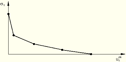
This fracture energy cracking model can be invoked by specifying the postfailure stress as a tabular function of cracking displacement, as shown in Figure 18.5.3–4.
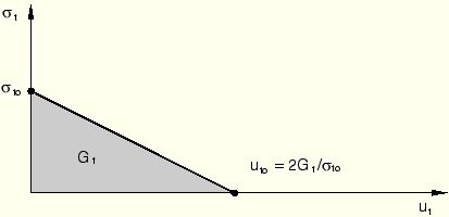
Alternatively, the fracture energy, ![]() , can be specified directly as a material property; in this case, define the failure stress,
, can be specified directly as a material property; in this case, define the failure stress, ![]() , as a tabular function of the associated fracture energy. This model assumes a linear loss of strength after cracking, as shown in Figure 18.5.3–5.
, as a tabular function of the associated fracture energy. This model assumes a linear loss of strength after cracking, as shown in Figure 18.5.3–5.
If tensile damage, ![]() , is specified, ABAQUS automatically converts the cracking displacement values to “plastic” displacement values using the relationship
, is specified, ABAQUS automatically converts the cracking displacement values to “plastic” displacement values using the relationship
![]()
The implementation of this stress-displacement concept in a finite element model requires the definition of a characteristic length associated with an integration point. The characteristic crack length is based on the element geometry: for beams and trusses we use the integration point length; for shell and planar elements we use the square root of the integration point area; for solid elements we use the cube root of the integration point volume. This definition of the characteristic crack length is used because the direction in which cracking occurs is not known in advance. Therefore, elements with large aspect ratios will have rather different behavior depending on the direction in which they crack: some mesh sensitivity remains because of this effect, and elements that have aspect ratios close to one are recommended.
| Input File Usage: | Use the following option to specify the postfailure stress as a tabular function of displacement: |
*CONCRETE TENSION STIFFENING, TYPE=DISPLACEMENT Use the following option to specify the postfailure stress as a tabular function of the fracture energy: *CONCRETE TENSION STIFFENING, TYPE=GFI |
| ABAQUS/CAE Usage: | Property module: material editor: Mechanical |
You can define the stress-strain behavior of plain concrete in uniaxial compression outside the elastic range. Compressive stress data are provided as a tabular function of inelastic (or crushing) strain, ![]() , and, if desired, strain rate, temperature, and field variables. Positive (absolute) values should be given for the compressive stress and strain. The stress-strain curve can be defined beyond the ultimate stress, into the strain-softening regime.
, and, if desired, strain rate, temperature, and field variables. Positive (absolute) values should be given for the compressive stress and strain. The stress-strain curve can be defined beyond the ultimate stress, into the strain-softening regime.
Hardening data are given in terms of an inelastic strain, ![]() , instead of plastic strain,
, instead of plastic strain, ![]() . The compressive inelastic strain is defined as the total strain minus the elastic strain corresponding to the undamaged material,
. The compressive inelastic strain is defined as the total strain minus the elastic strain corresponding to the undamaged material, ![]() , where
, where ![]() , as illustrated in Figure 18.5.3–6.
, as illustrated in Figure 18.5.3–6.
Figure 18.5.3–6 Definition of the compressive inelastic (or crushing) strain ![]() used for the definition of compression hardening data.
used for the definition of compression hardening data.

![]()
| Input File Usage: | *CONCRETE COMPRESSION HARDENING |
| ABAQUS/CAE Usage: | Property module: material editor: Mechanical |
Damage, ![]() and/or
and/or ![]() , can be specified in tabular form. (If damage is not specified, the model behaves as a plasticity model; consequently,
, can be specified in tabular form. (If damage is not specified, the model behaves as a plasticity model; consequently, ![]() and
and ![]() .)
.)
In ABAQUS the damage variables are treated as non-decreasing material point quantities. At any increment during the analysis, the new value of each damage variable is obtained as the maximum between the value at the end of the previous increment and the value corresponding to the current state (interpolated from the user-specified tabular data); that is,
The choice of the damage properties is important since, generally, excessive damage may have a critical effect on the rate of convergence. It is recommended to avoid using values of the damage variables above 0.99, which corresponds to a 99% reduction of the stiffness.
You can define the uniaxial tension damage variable, ![]() , as a tabular function of either cracking strain or cracking displacement.
, as a tabular function of either cracking strain or cracking displacement.
| Input File Usage: | Use the following option to specify tensile damage as a function of cracking strain: |
*CONCRETE TENSION DAMAGE, TYPE=STRAIN (default) Use the following option to specify tensile damage as a function of cracking displacement: *CONCRETE TENSION DAMAGE, TYPE=DISPLACEMENT |
| ABAQUS/CAE Usage: | Property module: material editor: Mechanical |
You can define the uniaxial compression damage variable, ![]() , as a tabular function of inelastic (crushing) strain.
, as a tabular function of inelastic (crushing) strain.
| Input File Usage: | *CONCRETE COMPRESSION DAMAGE |
| ABAQUS/CAE Usage: | Property module: material editor: Mechanical |
As discussed above, stiffness recovery is an important aspect of the mechanical response of concrete under cyclic loading. ABAQUS allows direct user specification of the stiffness recovery factors ![]() and
and ![]() .
.
The experimental observation in most quasi-brittle materials, including concrete, is that the compressive stiffness is recovered upon crack closure as the load changes from tension to compression. On the other hand, the tensile stiffness is not recovered as the load changes from compression to tension once crushing micro-cracks have developed. This behavior, which corresponds to ![]() and
and ![]() , is the default used by ABAQUS. Figure 18.5.3–7 illustrates a uniaxial load cycle assuming the default behavior.
, is the default used by ABAQUS. Figure 18.5.3–7 illustrates a uniaxial load cycle assuming the default behavior.
Figure 18.5.3–7 Uniaxial load cycle (tension-compression-tension) assuming default values for the stiffness recovery factors: ![]() and
and ![]() .
.
| Input File Usage: | Use the following option to specify the compression stiffness recovery factor, |
*CONCRETE TENSION DAMAGE, COMPRESSION RECOVERY= Use the following option to specify the tension stiffness recovery factor, *CONCRETE COMPRESSION DAMAGE, TENSION RECOVERY= |
| ABAQUS/CAE Usage: | Property module: material editor: Mechanical |
The rate-sensitive behavior of quasi-brittle materials is mainly connected to the retardation effects that high strain rates have on the growth of micro-cracks. The effect is usually more pronounced under tensile loading. As the strain rate increases, the stress-strain curves exhibit decreasing nonlinearity as well as an increase in the peak strength. You can specify tension stiffening as a tabular function of cracking strain (or displacement) rate, and you can specify compression hardening data as a tabular function of inelastic strain rate.
| Input File Usage: | Use the following options: |
*CONCRETE TENSION STIFFENING *CONCRETE COMPRESSION HARDENING |
| ABAQUS/CAE Usage: | Property module: material editor: Mechanical |
You can define flow potential, yield surface, and in ABAQUS/Standard viscosity parameters for the concrete damaged plasticity material model.
| Input File Usage: | *CONCRETE DAMAGED PLASTICITY |
| ABAQUS/CAE Usage: | Property module: material editor: Mechanical |
The effective stress is defined as
![]()
![]()
![]()
![]()
The concrete damaged plasticity model assumes nonassociated potential plastic flow. The flow potential G used for this model is the Drucker-Prager hyperbolic function:
![]()
![]()
is the dilation angle measured in the p–q plane at high confining pressure;
![]()
is the uniaxial tensile stress at failure, taken from the user-specified tension stiffening data; and
![]()
is a parameter, referred to as the eccentricity, that defines the rate at which the function approaches the asymptote (the flow potential tends to a straight line as the eccentricity tends to zero).
The default flow potential eccentricity is ![]() , which implies that the material has almost the same dilation angle over a wide range of confining pressure stress values. Increasing the value of
, which implies that the material has almost the same dilation angle over a wide range of confining pressure stress values. Increasing the value of ![]() provides more curvature to the flow potential, implying that the dilation angle increases more rapidly as the confining pressure decreases. Values of
provides more curvature to the flow potential, implying that the dilation angle increases more rapidly as the confining pressure decreases. Values of ![]() that are significantly less than the default value may lead to convergence problems if the material is subjected to low confining pressures because of the very tight curvature of the flow potential locally where it intersects the p-axis.
that are significantly less than the default value may lead to convergence problems if the material is subjected to low confining pressures because of the very tight curvature of the flow potential locally where it intersects the p-axis.
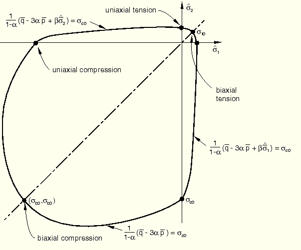
The model makes use of the yield function of Lubliner et. al. (1989), with the modifications proposed by Lee and Fenves (1998) to account for different evolution of strength under tension and compression. The evolution of the yield surface is controlled by the hardening variables, ![]() and
and ![]() . In terms of effective stresses, the yield function takes the form
. In terms of effective stresses, the yield function takes the form
![]()
![]()
is the maximum principal effective stress;
![]()
is the ratio of initial equibiaxial compressive yield stress to initial uniaxial compressive yield stress (the default value is ![]() );
);
![]()
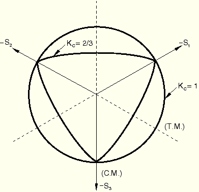
is the ratio of the second stress invariant on the tensile meridian, ![]() , to that on the compressive meridian,
, to that on the compressive meridian, ![]() , at initial yield for any given value of the pressure invariant p such that the maximum principal stress is negative,
, at initial yield for any given value of the pressure invariant p such that the maximum principal stress is negative, ![]() (see Figure 18.5.3–8); it must satisfy the condition
(see Figure 18.5.3–8); it must satisfy the condition ![]() (the default value is
(the default value is ![]() );
);
![]()
is the effective tensile cohesion stress; and
![]()
is the effective compressive cohesion stress.
Typical yield surfaces are shown in Figure 18.5.3–8 on the deviatoric plane and in Figure 18.5.3–9 for plane stress conditions.
Because plastic flow is nonassociated, the use of concrete damaged plasticity results in a nonsymmetric material stiffness matrix. Therefore, to obtain an acceptable rate of convergence in ABAQUS/Standard, the unsymmetric matrix storage and solution scheme should be used. ABAQUS/Standard will automatically activate the unsymmetric solution scheme if concrete damaged plasticity is used in the analysis. If desired, you can turn off the unsymmetric solution scheme for a particular step (see “Procedures: overview,” Section 6.1.1).
Material models exhibiting softening behavior and stiffness degradation often lead to severe convergence difficulties in implicit analysis programs, such as ABAQUS/Standard. A common technique to overcome some of these convergence difficulties is the use of a viscoplastic regularization of the constitutive equations, which causes the consistent tangent stiffness of the softening material to become positive for sufficiently small time increments.
The concrete damaged plasticity model can be regularized in ABAQUS/Standard using viscoplasticity by permitting stresses to be outside of the yield surface. We use a generalization of the Duvaut-Lions regularization, according to which the viscoplastic strain rate tensor, ![]() , is defined as
, is defined as
![]()
Similarly, a viscous stiffness degradation variable, ![]() , for the viscoplastic system is defined as
, for the viscoplastic system is defined as
![]()
![]()
Using the viscoplastic regularization with a small value for the viscosity parameter (small compared to the characteristic time increment) usually helps improve the rate of convergence of the model in the softening regime, without compromising results. The basic idea is that the solution of the viscoplastic system relaxes to that of the inviscid case as ![]() , where t represents time. You can specify the value of the viscosity parameter as part of the concrete damaged plasticity material behavior definition. If the viscosity parameter is different from zero, output results of the plastic strain and stiffness degradation refer to the viscoplastic values,
, where t represents time. You can specify the value of the viscosity parameter as part of the concrete damaged plasticity material behavior definition. If the viscosity parameter is different from zero, output results of the plastic strain and stiffness degradation refer to the viscoplastic values, ![]() and
and ![]() . In ABAQUS/Standard the default value of the viscosity parameter is zero, so that no viscoplastic regularization is performed.
. In ABAQUS/Standard the default value of the viscosity parameter is zero, so that no viscoplastic regularization is performed.
The concrete damaged plasticity model can be used in combination with material damping (see “Material damping,” Section 20.1.1). If stiffness proportional damping is specified, ABAQUS calculates the damping stress based on the undamaged elastic stiffness. This may introduce large artificial damping forces on elements undergoing severe damage at high strain rates.
Unlike concrete models based on the smeared crack approach, the concrete damaged plasticity model does not have the notion of cracks developing at the material integration point. However, it is possible to introduce the concept of an effective crack direction with the purpose of obtaining a graphical visualization of the cracking patterns in the concrete structure. Different criteria can be adopted within the framework of scalar-damage plasticity for the definition of the direction of cracking. Following Lubliner et. al. (1989), we can assume that cracking initiates at points where the tensile equivalent plastic strain is greater than zero, ![]() , and the maximum principal plastic strain is positive. The direction of the vector normal to the crack plane is assumed to be parallel to the direction of the maximum principal plastic strain. This direction can be viewed in the Visualization module of ABAQUS/CAE.
, and the maximum principal plastic strain is positive. The direction of the vector normal to the crack plane is assumed to be parallel to the direction of the maximum principal plastic strain. This direction can be viewed in the Visualization module of ABAQUS/CAE.
| ABAQUS/CAE Usage: | Visualization module:
Result |
ABAQUS offers a variety of elements for use with the concrete damaged plasticity model: truss, shell, plane stress, plane strain, generalized plane strain, axisymmetric, and three-dimensional elements. Most beam elements can be used; however, beam elements in space that include shear stress caused by torsion and do not include hoop stress (such as B31, B31H, B32, B32H, B33, and B33H) cannot be used. Thin-walled, open-section beam elements and PIPE elements can be used with the concrete damaged plasticity model.
For general shell analysis more than the default number of five integration points through the thickness of the shell should be used; nine thickness integration points are commonly used to model progressive failure of the concrete through the thickness with acceptable accuracy.
In addition to the standard output identifiers available in ABAQUS (“ABAQUS/Standard output variable identifiers,” Section 4.2.1, and “ABAQUS/Explicit output variable identifiers,” Section 4.2.2), the following variables relate specifically to material points in the concrete damaged plasticity model:
DAMAGEC | Compressive damage variable, |
DAMAGET | Tensile damage variable, |
PEEQ | Compressive equivalent plastic strain, |
PEEQT | Tensile equivalent plastic strain, |
SDEG | Stiffness degradation variable, d. |
DMENER | Energy dissipated per unit volume by damage. |
ELDMD | Total energy dissipated in the element by damage. |
ALLDMD | Energy dissipated in the whole (or partial) model by damage. The contribution from ALLDMD is included in the total strain energy ALLIE. |
EDMDDEN | Energy dissipated per unit volume in the element by damage. |
SENER | The recoverable part of the energy per unit volume. |
ELSE | The recoverable part of the energy in the element. |
ALLSE | The recoverable part of the energy in the whole (partial) model. |
ESEDEN | The recoverable part of the energy per unit volume in the element. |
Hillerborg, A., M. Modeer, and P. E. Petersson, “Analysis of Crack Formation and Crack Growth in Concrete by Means of Fracture Mechanics and Finite Elements,” Cement and Concrete Research, vol. 6, pp. 773–782, 1976.
Lee, J., and G. L. Fenves, “Plastic-Damage Model for Cyclic Loading of Concrete Structures,” Journal of Engineering Mechanics, vol. 124, no.8, pp. 892–900, 1998.
Lubliner, J., J. Oliver, S. Oller, and E. Oñate, “A Plastic-Damage Model for Concrete,” International Journal of Solids and Structures, vol. 25, pp. 299–329, 1989.