Products: ABAQUS/Standard ABAQUS/Explicit ABAQUS/CAE
The kinematic hardening models:
are used to simulate the inelastic behavior of materials that are subjected to cyclic loading;
include a linear kinematic hardening model and a nonlinear isotropic/kinematic hardening model;
can be used in any procedure that uses elements with displacement degrees of freedom;
in ABAQUS/Standard cannot be used in adiabatic analyses, and the nonlinear isotropic/kinematic hardening model cannot be used in coupled temperature-displacement analyses;
can be used to model rate-dependent yield;
can be used with creep and swelling in ABAQUS/Standard; and
require the use of the linear elasticity material model to define the elastic part of the response.
The kinematic hardening models used to model the behavior of metals subjected to cyclic loading are pressure-independent plasticity models; in other words, yielding of the metals is independent of the equivalent pressure stress. These models are suited for most metals subjected to cyclic loading conditions, except voided metals. The linear kinematic hardening model can be used with the Mises or Hill yield surface. The nonlinear isotropic/kinematic model can be used only with the Mises yield surface in ABAQUS/Standard and with the Mises or Hill yield surface in ABAQUS/Explicit. The pressure-independent yield surface is defined by the function
![]()
![]()
The kinematic hardening models assume associated plastic flow:
![]()
![]()
The linear kinematic hardening model has a constant hardening modulus, and the nonlinear isotropic/kinematic hardening model has both nonlinear kinematic and nonlinear isotropic hardening components.
The evolution law of this model consists of a linear kinematic hardening component that describes the translation of the yield surface in stress space through the backstress, ![]() . When temperature dependence is omitted, this evolution law is the linear Ziegler hardening law
. When temperature dependence is omitted, this evolution law is the linear Ziegler hardening law
![]()
The evolution law of this model consists of two components: a nonlinear kinematic hardening component, which describes the translation of the yield surface in stress space through the backstress, ![]() ; and an isotropic hardening component, which describes the change of the equivalent stress defining the size of the yield surface,
; and an isotropic hardening component, which describes the change of the equivalent stress defining the size of the yield surface, ![]() , as a function of plastic deformation.
, as a function of plastic deformation.
The kinematic hardening component is defined to be an additive combination of a purely kinematic term (linear Ziegler hardening law) and a relaxation term (the recall term), which introduces the nonlinearity. When temperature and field variable dependencies are omitted, the hardening law is
![]()
The isotropic hardening behavior of the model defines the evolution of the yield surface size, ![]() , as a function of the equivalent plastic strain,
, as a function of the equivalent plastic strain, ![]() . This evolution can be introduced by specifying
. This evolution can be introduced by specifying ![]() directly as a function of
directly as a function of ![]() in tabular form, by specifying
in tabular form, by specifying ![]() in user subroutine UHARD (in ABAQUS/Standard only), or by using the simple exponential law
in user subroutine UHARD (in ABAQUS/Standard only), or by using the simple exponential law
![]()
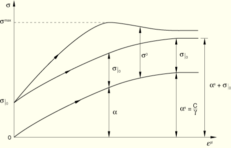
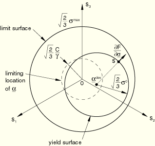
The evolution of the kinematic and the isotropic hardening components is illustrated in Figure 18.2.2–1 for unidirectional loading and in Figure 18.2.2–2 for multiaxial loading. The evolution law for the kinematic hardening component implies that the backstress is contained within a cylinder of radius ![]() , where
, where ![]() is the magnitude of
is the magnitude of ![]() at saturation (large plastic strains). It also implies that any stress point must lie within a cylinder of radius
at saturation (large plastic strains). It also implies that any stress point must lie within a cylinder of radius ![]() (using the notation of Figure 18.2.2–1) since the yield surface remains bounded. At large plastic strain any stress point is contained within a cylinder of radius
(using the notation of Figure 18.2.2–1) since the yield surface remains bounded. At large plastic strain any stress point is contained within a cylinder of radius ![]() , where
, where ![]() is the equivalent stress defining the size of the yield surface at large plastic strain. If tabular data are provided for the isotropic component,
is the equivalent stress defining the size of the yield surface at large plastic strain. If tabular data are provided for the isotropic component, ![]() is the last value given to define the size of the yield surface. If user subroutine UHARD is used, this value will depend on your implementation; otherwise,
is the last value given to define the size of the yield surface. If user subroutine UHARD is used, this value will depend on your implementation; otherwise, ![]() .
.
In the kinematic hardening models the center of the yield surface moves in stress space due to the kinematic hardening component. In addition, when the nonlinear isotropic/kinematic hardening model is used, the yield surface range may expand or contract due to the isotropic component. These features allow modeling of inelastic deformation in metals that are subjected to cycles of load or temperature, resulting in significant inelastic deformation and, possibly, low-cycle fatigue failure. These models account for the following phenomena:
Bauschinger effect: This effect is characterized by a reduced yield stress upon load reversal after plastic deformation has occurred during the initial loading. This phenomenon decreases with continued cycling. The linear kinematic hardening component takes this effect into consideration, but a nonlinear component improves the shape of the cycles.
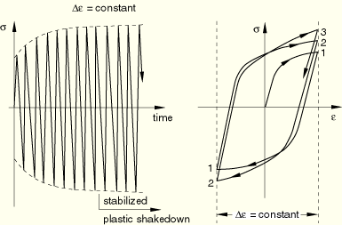
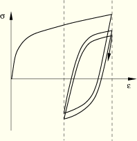
Cyclic hardening with plastic shakedown: This phenomenon is characteristic of symmetric stress- or strain-controlled experiments. Soft or annealed metals tend to harden toward a stable limit, and initially hardened metals tend to soften. Figure 18.2.2–3 illustrates the behavior of a metal that hardens under prescribed symmetric strain cycles.
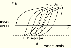
The kinematic hardening component of the models used alone predicts plastic shakedown after one stress cycle. The combination of the isotropic component together with the nonlinear kinematic component predicts shakedown after several cycles.Ratchetting: Unsymmetric cycles of stress between prescribed limits will cause progressive “creep” or “ratchetting” in the direction of the mean stress (Figure 18.2.2–4).
Typically, transient ratchetting is followed by stabilization (zero ratchet strain) for low mean stresses, while a constant increase in the accumulated ratchet strain is observed at high mean stresses. The nonlinear kinematic hardening component, used without the isotropic hardening component, predicts constant ratchet strain. The prediction of ratchetting is improved by adding isotropic hardening, in which case the ratchet strain may decrease until it becomes constant.Relaxation of the mean stress: This phenomenon is characteristic of an unsymmetric strain experiment, as shown in Figure 18.2.2–5.
As the number of cycles increases, the mean stress tends to zero. The nonlinear kinematic hardening component of the nonlinear isotropic/kinematic hardening model accounts for this behavior.The linear kinematic model is a simple model that gives only a first approximation of the behavior of metals subjected to cyclic loading, as explained above. The nonlinear isotropic/kinematic hardening model can provide more accurate results in many cases involving cyclic loading, but it still has the following limitations:
The isotropic hardening is the same at all strain ranges. Physical observations, however, indicate that the amount of isotropic hardening depends on the magnitude of the strain range. Furthermore, if the specimen is cycled at two different strain ranges, one followed by the other, the deformation in the first cycle affects the isotropic hardening in the second cycle. Thus, the model is only a coarse approximation of actual cyclic behavior. It should be calibrated to the expected size of the strain cycles of importance in the application.
The same cyclic hardening behavior is predicted for proportional and nonproportional load cycles. Physical observations indicate that the cyclic hardening behavior of materials subjected to nonproportional loading may be very different from uniaxial behavior at a similar strain amplitude.
The linear kinematic model approximates the hardening behavior with a constant rate of hardening. This hardening rate should be matched to the average hardening rate measured in stabilized cycles over a strain range corresponding to that expected in the application. A stabilized cycle is obtained by cycling over a fixed strain range until a steady-state condition is reached; that is, until the stress-strain curve no longer changes shape from one cycle to the next. The more general nonlinear model will give better predictions but requires more detailed calibration.
The test data obtained from a half cycle of a unidirectional tension or compression experiment must be linearized, since this simple model can predict only linear hardening. The data are usually based on measurements of the stabilized behavior in strain cycles covering a strain range corresponding to the strain range that is anticipated to occur in the application. ABAQUS expects you to provide only two data pairs to define this linear behavior: the yield stress, ![]() , at zero plastic strain and a yield stress,
, at zero plastic strain and a yield stress, ![]() , at a finite plastic strain value,
, at a finite plastic strain value, ![]() . The linear kinematic hardening modulus, C, is determined from the relation
. The linear kinematic hardening modulus, C, is determined from the relation
![]()
You can provide several sets of two data pairs as a function of temperature to define the variation of the linear kinematic hardening modulus with respect to temperature. If the Hill yield surface is desired for this model, you must specify a set of yield ratios, ![]() , independently (see “Anisotropic yield/creep,” Section 18.2.6, for information on how to specify the yield ratios).
, independently (see “Anisotropic yield/creep,” Section 18.2.6, for information on how to specify the yield ratios).
This model gives physically reasonable results for only relatively small strains (less than 5%).
| Input File Usage: | *PLASTIC, HARDENING=KINEMATIC |
| ABAQUS/CAE Usage: | Property module: material editor: Mechanical |
The evolution of the equivalent stress defining the size of the yield surface, ![]() , as a function of the equivalent plastic strain,
, as a function of the equivalent plastic strain, ![]() , defines the isotropic hardening component of the model. You can define this isotropic hardening component through an exponential law or directly in tabular form. It need not be defined if the yield surface remains fixed throughout the loading. In ABAQUS/Explicit if the Hill yield surface is desired for this model, you must specify a set of yield ratios,
, defines the isotropic hardening component of the model. You can define this isotropic hardening component through an exponential law or directly in tabular form. It need not be defined if the yield surface remains fixed throughout the loading. In ABAQUS/Explicit if the Hill yield surface is desired for this model, you must specify a set of yield ratios, ![]() , independently (see “Anisotropic yield/creep,” Section 18.2.6, for information on how to specify the yield ratios). The Hill yield surface cannot be used with this model in ABAQUS/Standard.
, independently (see “Anisotropic yield/creep,” Section 18.2.6, for information on how to specify the yield ratios). The Hill yield surface cannot be used with this model in ABAQUS/Standard.
The material parameters C and ![]() determine the kinematic hardening component of the model. ABAQUS offers three different ways of providing data for the kinematic hardening component of the model: the parameters C and
determine the kinematic hardening component of the model. ABAQUS offers three different ways of providing data for the kinematic hardening component of the model: the parameters C and ![]() can be specified directly, half-cycle test data can be given, or test data obtained from a stabilized cycle can be given. The experiments required to calibrate the model are described below.
can be specified directly, half-cycle test data can be given, or test data obtained from a stabilized cycle can be given. The experiments required to calibrate the model are described below.
Specify the material parameters of the exponential law ![]() ,
, ![]() , and b directly if they are already calibrated from test data. These parameters can be specified as functions of temperature and/or field variables.
, and b directly if they are already calibrated from test data. These parameters can be specified as functions of temperature and/or field variables.
| Input File Usage: | *CYCLIC HARDENING, PARAMETERS |
| ABAQUS/CAE Usage: | Property module: material editor: Mechanical |
Isotropic hardening can be introduced by specifying the equivalent stress defining the size of the yield surface, ![]() , as a tabular function of the equivalent plastic strain,
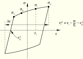
, as a tabular function of the equivalent plastic strain, ![]() . The simplest way to obtain these data is to conduct a symmetric strain-controlled cyclic experiment with strain range
. The simplest way to obtain these data is to conduct a symmetric strain-controlled cyclic experiment with strain range ![]() . Since the material's elastic modulus is large compared to its hardening modulus, this experiment can be interpreted approximately as repeated cycles over the same plastic strain range
. Since the material's elastic modulus is large compared to its hardening modulus, this experiment can be interpreted approximately as repeated cycles over the same plastic strain range ![]() (using the notation of Figure 18.2.2–6, where E is the Young's modulus of the material).
(using the notation of Figure 18.2.2–6, where E is the Young's modulus of the material).
![]()
![]()
Data pairs (![]() ,
, ![]() ), including the value
), including the value ![]() at zero equivalent plastic strain, are specified in tabulated form. The tabulated values defining the size of the yield surface should be provided for the entire equivalent plastic strain range to which the material may be subjected. The data can be provided as functions of temperature and/or field variables.
at zero equivalent plastic strain, are specified in tabulated form. The tabulated values defining the size of the yield surface should be provided for the entire equivalent plastic strain range to which the material may be subjected. The data can be provided as functions of temperature and/or field variables.
To obtain accurate cyclic hardening data, such as would be needed for low-cycle fatigue calculations, the calibration experiment should be performed at a strain range, ![]() , that corresponds to the strain range anticipated in the analysis because the material model does not predict different isotropic hardening behavior at different strain ranges. This limitation also implies that, even though a component is made from the same material, it may have to be divided into several regions with different hardening properties corresponding to different anticipated strain ranges. Field variables and field variable dependence of these properties can also be used for this purpose.
, that corresponds to the strain range anticipated in the analysis because the material model does not predict different isotropic hardening behavior at different strain ranges. This limitation also implies that, even though a component is made from the same material, it may have to be divided into several regions with different hardening properties corresponding to different anticipated strain ranges. Field variables and field variable dependence of these properties can also be used for this purpose.
ABAQUS allows the specification of strain rate effects in the isotropic component of the nonlinear isotropic/kinematic hardening model. The rate-dependent isotropic hardening data can be defined by specifying the equivalent stress defining the size of the yield surface, ![]() , as a tabular function of the equivalent plastic strain,
, as a tabular function of the equivalent plastic strain, ![]() , at different values of the equivalent plastic strain rate,
, at different values of the equivalent plastic strain rate, ![]() .
.
| Input File Usage: | Use the following option to define isotropic hardening with tabular data: |
*CYCLIC HARDENING Use the following option to define rate-dependent isotropic hardening with tabular data: *CYCLIC HARDENING, RATE= |
| ABAQUS/CAE Usage: | Property module: material editor: Mechanical |
Specify ![]() directly in user subroutine UHARD.
directly in user subroutine UHARD. ![]() may be dependent on equivalent plastic strain and temperature. This method cannot be used if the kinematic hardening component is specified by using half-cycle test data.
may be dependent on equivalent plastic strain and temperature. This method cannot be used if the kinematic hardening component is specified by using half-cycle test data.
| Input File Usage: | *CYCLIC HARDENING, USER |
| ABAQUS/CAE Usage: | Property module: material editor: Mechanical |
The parameters C and ![]() can be specified directly if they are already calibrated from test data. The parameter C can be provided as a function of temperature and/or field variables, but temperature and field variable dependence of
can be specified directly if they are already calibrated from test data. The parameter C can be provided as a function of temperature and/or field variables, but temperature and field variable dependence of ![]() is not available. The algorithm currently used to integrate the nonlinear isotropic/kinematic hardening model does not provide accurate solutions if the value of
is not available. The algorithm currently used to integrate the nonlinear isotropic/kinematic hardening model does not provide accurate solutions if the value of ![]() changes significantly in an increment due to temperature and/or field variable dependence.
changes significantly in an increment due to temperature and/or field variable dependence.
| Input File Usage: | *PLASTIC, HARDENING=COMBINED, DATA TYPE=PARAMETERS |
| ABAQUS/CAE Usage: | Property module: material editor: Mechanical |
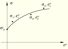
If limited test data are available, C and ![]() can be based on the stress-strain data obtained from the first half cycle of a unidirectional tension or compression experiment. An example of such test data is shown in Figure 18.2.2–7. This approach is usually adequate when the simulation will involve only a few cycles of loading.
can be based on the stress-strain data obtained from the first half cycle of a unidirectional tension or compression experiment. An example of such test data is shown in Figure 18.2.2–7. This approach is usually adequate when the simulation will involve only a few cycles of loading.
For each data point (![]() ) a value of
) a value of ![]() is obtained from the test data as
is obtained from the test data as
![]()
Integration of the backstress evolution law over a half cycle yields the expression
![]()
When test data are given as functions of temperature and/or field variables, it is recommended that a data check analysis be run first. During the data check run, ABAQUS will determine several pairs of material parameters (C, ![]() ), where each pair will correspond to a given combination of temperature and/or field variables. Since ABAQUS requires the parameter
), where each pair will correspond to a given combination of temperature and/or field variables. Since ABAQUS requires the parameter ![]() to be a constant, the data check analysis will terminate with an error message if
to be a constant, the data check analysis will terminate with an error message if ![]() is not a constant. However, an appropriate constant value of
is not a constant. However, an appropriate constant value of ![]() may be determined from the information provided in the data file during the data check run. The values for the parameters C and the constant
may be determined from the information provided in the data file during the data check run. The values for the parameters C and the constant ![]() can then be entered directly as described above.
can then be entered directly as described above.
| Input File Usage: | *PLASTIC, HARDENING=COMBINED, DATA TYPE=HALF CYCLE |
| ABAQUS/CAE Usage: | Property module: material editor: Mechanical |
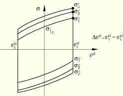
Stress-strain data can be obtained from the stabilized cycle of a specimen that is subjected to symmetric strain cycles. A stabilized cycle is obtained by cycling the specimen over a fixed strain range ![]() until a steady-state condition is reached; that is, until the stress-strain curve no longer changes shape from one cycle to the next. Such a stabilized cycle is shown in Figure 18.2.2–8.
until a steady-state condition is reached; that is, until the stress-strain curve no longer changes shape from one cycle to the next. Such a stabilized cycle is shown in Figure 18.2.2–8.
![]()
For each pair (![]() ) values of
) values of ![]() are obtained from the test data as
are obtained from the test data as
![]()
Integration of the backstress evolution law over this uniaxial strain cycle, with an exact match for the first data pair (![]() ), provides the expression
), provides the expression
![]()
If the shapes of the stress-strain curves are significantly different for different strain ranges, you may want to obtain several calibrated values of C and ![]() . The tabular data of the stress-strain curves obtained at different strain ranges can be entered directly in ABAQUS. Calibrated values corresponding to each strain range are reported in the data file, together with an averaged set of parameters, if model definition data are requested (see “Controlling the amount of analysis input file processor information written to the data file” in “Output,” Section 4.1.1). ABAQUS will use the averaged set in the analysis. These parameters may have to be adjusted to improve the match to the test data at the strain range anticipated in the analysis.
. The tabular data of the stress-strain curves obtained at different strain ranges can be entered directly in ABAQUS. Calibrated values corresponding to each strain range are reported in the data file, together with an averaged set of parameters, if model definition data are requested (see “Controlling the amount of analysis input file processor information written to the data file” in “Output,” Section 4.1.1). ABAQUS will use the averaged set in the analysis. These parameters may have to be adjusted to improve the match to the test data at the strain range anticipated in the analysis.
When test data are given as functions of temperature and/or field variables, it is recommended that a data check analysis be run first. During the data check run, ABAQUS will determine several pairs of material parameters (C, ![]() ), where each pair will correspond to a given combination of temperature and/or field variables. Since ABAQUS requires the parameter
), where each pair will correspond to a given combination of temperature and/or field variables. Since ABAQUS requires the parameter ![]() to be a constant, the data check analysis will terminate with an error message if
to be a constant, the data check analysis will terminate with an error message if ![]() is not a constant. However, an appropriate constant value of
is not a constant. However, an appropriate constant value of ![]() may be determined from the information provided in the data file during the data check run. The values for the parameters C and the constant
may be determined from the information provided in the data file during the data check run. The values for the parameters C and the constant ![]() can then be entered directly as described above.
can then be entered directly as described above.
The isotropic hardening component should be defined by specifying the equivalent stress defining the size of the yield surface at zero plastic strain, as well as the evolution of the equivalent stress as a function of equivalent plastic strain. If this component is not defined, ABAQUS will assume that no cyclic hardening occurs so that the equivalent stress defining the size of the yield surface is constant and equal to ![]() (or the average of these quantities over several strain ranges when more than one strain range is provided). Since this size corresponds to the size of a saturated cycle, this is unlikely to provide accurate predictions of actual behavior, particularly in the initial cycles.
(or the average of these quantities over several strain ranges when more than one strain range is provided). Since this size corresponds to the size of a saturated cycle, this is unlikely to provide accurate predictions of actual behavior, particularly in the initial cycles.
| Input File Usage: | *PLASTIC, HARDENING=COMBINED, DATA TYPE=STABILIZED |
| ABAQUS/CAE Usage: | Property module: material editor: Mechanical |
There are cases when we need to study the behavior of a material that has already been subjected to some hardening. For such cases ABAQUS allows you to prescribe initial conditions for the equivalent plastic strain, ![]() , and for the backstress,
, and for the backstress, ![]() . When the nonlinear isotropic/kinematic hardening model is used, the initial condition for the backstress,
. When the nonlinear isotropic/kinematic hardening model is used, the initial condition for the backstress, ![]() , must satisfy the condition
, must satisfy the condition
![]()
You can specify the initial values of ![]() and
and ![]() directly as initial conditions (see “Initial conditions,” Section 27.2.1).
directly as initial conditions (see “Initial conditions,” Section 27.2.1).
| Input File Usage: | *INITIAL CONDITIONS, TYPE=HARDENING |
| ABAQUS/CAE Usage: | Initial hardening conditions are not supported in ABAQUS/CAE. |
For more complicated cases in ABAQUS/Standard initial conditions can be defined through user subroutine HARDINI.
| Input File Usage: | *INITIAL CONDITIONS, TYPE=HARDENING, USER |
| ABAQUS/CAE Usage: | User subroutine HARDINI is not supported in ABAQUS/CAE. |
These models can be used with elements in ABAQUS/Standard that include mechanical behavior (elements that have displacement degrees of freedom), except some beam elements in space. Beam elements in space that include shear stress caused by torsion (i.e., not thin-walled, open sections) and do not include hoop stress (i.e., not PIPE elements) cannot be used. In ABAQUS/Explicit the kinematic hardening models can be used with any elements that include mechanical behavior, with the exception of one-dimensional elements (beams and trusses) when the models are used with the Hill yield surface.
In addition to the standard output identifiers available in ABAQUS (“ABAQUS/Standard output variable identifiers,” Section 4.2.1, and “ABAQUS/Explicit output variable identifiers,” Section 4.2.2), the following variables have special meaning for the kinematic hardening models:
ALPHA | Kinematic hardening shift tensor components, |
PEEQ | Equivalent plastic strain, |
PENER | Plastic work, defined as: |