Products: ABAQUS/Standard ABAQUS/Explicit
The Mullins effect model:
is intended for modeling stress softening of filled rubber elastomers under quasi-static cyclic loading, a phenomenon referred to in the literature as Mullins effect;
provides an extension to the well-known isotropic hyperelastic models;
is based on the theory of incompressible isotropic elasticity modified by the addition of a single variable, referred to as the damage variable;
assumes that only the deviatoric part of the material response is associated with damage;
is intended for modeling material response in situations where different parts of the model undergo different levels of damage resulting in a different material response; and
cannot be used with viscoelasticity or hysteresis.
The real behavior of filled rubber elastomers under cyclic loading conditions is quite complex. Certain idealizations have been made for modeling purposes. In essence, these idealizations result in two main components to the material behavior: the first component describes the response of a material point (from an undeformed state) under monotonic straining, and the second component is associated with damage and describes the unloading-reloading behavior. The idealized response and the two components are described in the following sections.
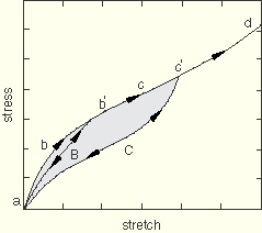
When an elastomeric test specimen is subjected to simple tension from its virgin state, unloaded, and then reloaded, the stress required on reloading is less than that on the initial loading for stretches up to the maximum stretch achieved during the initial loading. This stress softening phenomenon is known as the Mullins effect and reflects damage incurred during previous loading. This type of material response is depicted qualitatively in Figure 17.6.1–1.
This figure and the accompanying description is based on work by Ogden and Roxburgh (1999), which forms the basis of the model implemented in ABAQUS. Consider the primary loading pathThis is an ideal representation of Mullins effect since in practice there is some permanent set upon unloading and/or viscoelastic effects such as hysteresis. Points such as ![]() and
and ![]() may not exist in reality in the sense that unloading from the primary curve followed by reloading to the maximum strain level attained earlier usually results in a stress that is somewhat lower than the stress corresponding to the primary curve. In addition, the cyclic response for some filled elastomers shows evidence of progressive damage during unloading from and subsequent reloading to a certain maximum strain level. Such progressive damage usually occurs during the first few cycles, and the material behavior soon stabilizes to a loading/unloading cycle that is followed beyond the first few cycles. More details regarding the actual behavior and how test data that display such behavior can be used to calibrate the ABAQUS model for Mullins effect are discussed later and in “Analysis of a solid disc with Mullins effect,” Section 3.1.7 of the ABAQUS Example Problems Manual.
may not exist in reality in the sense that unloading from the primary curve followed by reloading to the maximum strain level attained earlier usually results in a stress that is somewhat lower than the stress corresponding to the primary curve. In addition, the cyclic response for some filled elastomers shows evidence of progressive damage during unloading from and subsequent reloading to a certain maximum strain level. Such progressive damage usually occurs during the first few cycles, and the material behavior soon stabilizes to a loading/unloading cycle that is followed beyond the first few cycles. More details regarding the actual behavior and how test data that display such behavior can be used to calibrate the ABAQUS model for Mullins effect are discussed later and in “Analysis of a solid disc with Mullins effect,” Section 3.1.7 of the ABAQUS Example Problems Manual.
The loading path ![]() will henceforth be referred to as the “primary hyperelastic behavior.” The primary hyperelastic behavior is defined by using a hyperelastic material model.
will henceforth be referred to as the “primary hyperelastic behavior.” The primary hyperelastic behavior is defined by using a hyperelastic material model.
Stress softening is interpreted as being due to damage at the microscopic level. As the material is loaded, the damage occurs by the severing of bonds between filler particles and the rubber molecular chains. Different chain links break at different deformation levels, thereby leading to continuous damage with macroscopic deformation. An equivalent interpretation is that the energy required to cause the damage is not recoverable.
Hyperelastic materials are described in terms of a “strain energy potential” function ![]() that defines the strain energy stored in the material per unit reference volume (volume in the initial configuration). The quantity
that defines the strain energy stored in the material per unit reference volume (volume in the initial configuration). The quantity ![]() is the deformation gradient tensor. To account for Mullins effect, Ogden and Roxburgh propose a material description that is based on an energy function of the form
is the deformation gradient tensor. To account for Mullins effect, Ogden and Roxburgh propose a material description that is based on an energy function of the form ![]() , where the additional scalar variable,
, where the additional scalar variable, ![]() , represents damage in the material. The damage variable controls the material properties in the sense that it enables the material response to be governed by an energy function on unloading and subsequent submaximal reloading different from that on the primary (initial) loading path from a virgin state. Because of the above interpretation of
, represents damage in the material. The damage variable controls the material properties in the sense that it enables the material response to be governed by an energy function on unloading and subsequent submaximal reloading different from that on the primary (initial) loading path from a virgin state. Because of the above interpretation of ![]() , it is no longer appropriate to think of U as the stored elastic energy potential. Part of the energy is stored as strain energy, while the rest is dissipated due to damage. The shaded area in Figure 17.6.1–1 represents the energy dissipated by damage as a result of deformation until the point
, it is no longer appropriate to think of U as the stored elastic energy potential. Part of the energy is stored as strain energy, while the rest is dissipated due to damage. The shaded area in Figure 17.6.1–1 represents the energy dissipated by damage as a result of deformation until the point ![]() , while the unshaded part represents the recoverable strain energy.
, while the unshaded part represents the recoverable strain energy.
The following paragraphs provide a summary of the Mullins effect model in ABAQUS. For further details, see “Mullins effect,” Section 4.7.1 of the ABAQUS Theory Manual. In preparation for writing the constitutive equations for Mullins effect, it is useful to separate the deviatoric and the volumetric parts of the total strain energy density as
![]()
The Mullins effect is accounted for by using an augmented energy function of the form
![]()
With the above modification to the energy function, the stresses are given by
![]()
The damage variable, ![]() , varies with the deformation according to
, varies with the deformation according to
![]()
![]()
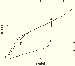
If the parameter ![]() and the parameter m has a value that is small compared to
and the parameter m has a value that is small compared to ![]() , the slope of the stress-strain curve at the initiation of unloading from relatively large strain levels may become very high. As a result, the response may become discontinuous, as illustrated in Figure 17.6.1–2.
, the slope of the stress-strain curve at the initiation of unloading from relatively large strain levels may become very high. As a result, the response may become discontinuous, as illustrated in Figure 17.6.1–2.
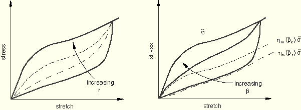
The parameters r, ![]() , and m do not have direct physical interpretations in general. The parameter m controls whether damage occurs at low strain levels. If
, and m do not have direct physical interpretations in general. The parameter m controls whether damage occurs at low strain levels. If ![]() , there is a significant amount of damage at low strain levels. On the other hand, a nonzero m leads to little or no damage at low strain levels. For further discussion regarding the implications of this model to the energy dissipation, see “Mullins effect,” Section 4.7.1 of the ABAQUS Theory Manual. The qualitative effects of varying the parameters r and
, there is a significant amount of damage at low strain levels. On the other hand, a nonzero m leads to little or no damage at low strain levels. For further discussion regarding the implications of this model to the energy dissipation, see “Mullins effect,” Section 4.7.1 of the ABAQUS Theory Manual. The qualitative effects of varying the parameters r and ![]() individually, while holding the other parameters fixed, are shown in Figure 17.6.1–3.
individually, while holding the other parameters fixed, are shown in Figure 17.6.1–3.
![]()
The primary hyperelastic behavior is defined by using the hyperelastic material model (see “Hyperelastic behavior of rubberlike materials,” Section 17.5.1). The Mullins effect model can be defined by specifying the Mullins effect parameters directly or by using test data to calibrate the parameters. Alternatively, in ABAQUS/Standard user subroutine UMULLINS can be used.
The parameters r, m, and ![]() of the Mullins effect can be given directly as functions of temperature and/or field variables.
of the Mullins effect can be given directly as functions of temperature and/or field variables.
| Input File Usage: | *MULLINS EFFECT |
Experimental unloading-reloading data from different strain levels can be specified for up to three simple tests: uniaxial, biaxial, and planar. ABAQUS will then compute the material parameters using a nonlinear least-squares curve fitting algorithm. It is generally best to obtain data from several experiments involving different kinds of deformation over the range of strains of interest in the actual application and to use all these data to determine the parameters. It is also important to obtain a good curve-fit for the primary hyperelastic behavior if the primary behavior is defined using test data.
By default, ABAQUS attempts to fit all three parameters to the given data. This is possible in general, except in the situation when the test data correspond to unloading-reloading from only a single value of ![]() . In this case the parameters m and
. In this case the parameters m and ![]() cannot be determined independently; one of them must be specified. If you specify neither m nor
cannot be determined independently; one of them must be specified. If you specify neither m nor ![]() , ABAQUS needs to assume a default value for one of these parameters. In light of the potential problems discussed earlier with
, ABAQUS needs to assume a default value for one of these parameters. In light of the potential problems discussed earlier with ![]() , ABAQUS assumes that
, ABAQUS assumes that ![]() in the above situation. The curve-fitting may also be carried out by specifying any one or two of the material parameters to be fixed, predetermined values.
in the above situation. The curve-fitting may also be carried out by specifying any one or two of the material parameters to be fixed, predetermined values.
As many data points as required can be entered from each test. It is recommended that data from all three tests (on samples taken from the same piece of material) be included and that the data points cover unloading/reloading from/to the range of nominal strain expected to arise in the actual loading.
The strain data should be given as nominal strain values (change in length per unit of original length). The stress data should be given as nominal stress values (force per unit of original cross-sectional area). These tests allow for entering both compression and tension data. Compressive stresses and strains are entered as negative values.
For each set of test input, the data point with the maximum nominal strain identifies the point of unloading. This point is used by the curve-fitting algorithm to compute ![]() for that curve.
for that curve.
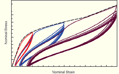
Figure 17.6.1–4 shows some typical unloading-reloading data from three different strain levels.
The data include multiple loading and unloading cycles from each strain level. As Figure 17.6.1–4 indicates, the loading/unloading cycles from any given strain level do not occur along a single curve, and there is some amount of hysteresis. There is also some amount of permanent set upon removal of the applied load. The data also show evidence of progressive damage with repeated cycling at any given maximum strain level. The response appears to stabilize after a number of cycles. When such data are used to calibrate the Mullins effect model, the resulting response will capture the overall stiffness characteristics, while ignoring effects such as hysteresis, permanent set, or progressive damage. The above data can be provided to ABAQUS in the following manner:The primary curve can be made up of the data points indicated by the dashed curve in Figure 17.6.1–4. Essentially, this consists of an envelope of the first loading curves to the different strain levels.
The unloading-reloading curves from the three different strain levels can be specified by providing the data points as is; i.e., as the repeated unloading-reloading cycles shown in Figure 17.6.1–4. As discussed earlier, the data from the different strain levels need to be distinguished by providing them as different tables. For example, assuming that the test data correspond to the uniaxial tension state, three tables of uniaxial test data would have to be defined for the three different strain levels shown in Figure 17.6.1–4. In this case ABAQUS will provide a best fit using all the data points (from all strain levels). The resulting fit would result in a response that is an average of all the test data at any given strain level. Both the hysteresis and the permanent set will be lost in the process.
Alternatively, you may provide any one unloading-reloading cycle from each different strain level. If the component is expected to undergo repeated cyclic loading, the latter may be, for example, the stabilized cycle at each strain level. On the other hand, if the component is expected to undergo predominantly monotonic loading with perhaps small amounts of unloading, the very first unloading curve at each strain level may be the appropriate input data for calibrating the Mullins coefficients.
Once the Mullins effect constants are determined, the behavior of the Mullins effect model in ABAQUS is established. However, the quality of this behavior must be assessed: the prediction of material behavior under different deformation modes must be compared against the experimental data. You must judge whether the Mullins effect constants determined by ABAQUS are acceptable, based on the correlation between the ABAQUS predictions and the experimental data. Single-element test cases can be used to derive the nominal stress–nominal strain response of the material model.
The steps that can be taken for improving the quality of the fit for the Mullins effect parameters are similar in essence to the guidelines provided for curve fitting the primary hyperelastic behavior (see “Hyperelastic behavior of rubberlike materials,” Section 17.5.1, for details). In addition, the quality of the fit for the Mullins effect parameters depends on a good fit for the primary hyperelastic behavior, if the primary behavior is defined using test data.
The quality of the fit can be evaluated by carrying out a numerical experiment with a single element that is loaded in the same mode for which test data has been provided. Alternatively, the numerical response for both the primary and the softening behavior can be obtained by requesting model definition data output (see “Output,” Section 4.1.1) and carrying out a data check analysis. The response computed by ABAQUS is printed in the data (.dat) file along with the experimental data. This tabular data can be plotted in ABAQUS/CAE for comparison and evaluation purposes. The primary hyperelastic behavior can also be evaluated with the automated material evaluation tools in ABAQUS/CAE.
| Input File Usage: | *MULLINS EFFECT, TEST DATA INPUT, BETA and/or M and/or R |
In addition, use at least one and up to three of the following options to give the unloading-reloading test data (see “Experimental tests” in the section describing hyperelastic test data input, “Hyperelastic behavior of rubberlike materials,” Section 17.5.1): *UNIAXIAL TEST DATA *BIAXIAL TEST DATA *PLANAR TEST DATA Multiple unloading-reloading curves from different strain levels for any given test type can be entered by repeated specification of the appropriate test data option. |
An alternative method provided in ABAQUS/Standard for defining the Mullins effect involves defining the damage variable in user subroutine UMULLINS. Optionally, you can specify the number of property values needed as data in the user subroutine. You must provide the damage variable, ![]() , and its derivative,
, and its derivative, ![]() . The latter contributes to the Jacobian of the overall system of equations and is necessary to ensure good convergence characteristics. If needed, you can specify the number of solution-dependent variables (“User subroutines: overview,” Section 13.2.1). These solution-dependent variables can be updated in the user subroutine. The damage dissipation energy and the recoverable part of the energy may also be defined for output purposes.
. The latter contributes to the Jacobian of the overall system of equations and is necessary to ensure good convergence characteristics. If needed, you can specify the number of solution-dependent variables (“User subroutines: overview,” Section 13.2.1). These solution-dependent variables can be updated in the user subroutine. The damage dissipation energy and the recoverable part of the energy may also be defined for output purposes.
The Ogden-Roxburgh framework of modeling the Mullins effect requires that the damage variable ![]() be defined as a monotonically increasing function of
be defined as a monotonically increasing function of ![]() .
.
User subroutine UMULLINS can be used in combination with all hyperelastic potentials in ABAQUS/Standard, including a user-defined potential (user subroutine UHYPER).
| Input File Usage: | *MULLINS EFFECT, USER, PROPERTIES=constants |
The Mullins effect material model can be used with all element types that support the use of the hyperelastic material model.
The Mullins effect material model can be used in all procedure types that support the use of the hyperelastic material model. In linear perturbation steps in ABAQUS/Standard the current material tangent stiffness is used to determine the response. Specifically, when a linear perturbation is carried out about a base state that is on the primary curve, the unloading tangent stiffness will be used.
In ABAQUS/Explicit the unloading tangent stiffness is always used to compute the stable time increment. As a result, the inclusion of Mullins effect leads to more increments in the analysis, even when no unloading actually takes place.
The Mullins effect material model can also be used in a steady-state transport analysis in ABAQUS/Standard to obtain steady-state rolling solutions. Issues related to the use of the Mullins effect in a steady-state transport analysis can be found in “Steady-state transport analysis,” Section 6.4.1, and “Analysis of a solid disc with Mullins effect,” Section 3.1.7 of the ABAQUS Example Problems Manual.
In addition to the standard output identifiers available in ABAQUS (“ABAQUS/Standard output variable identifiers,” Section 4.2.1, and “ABAQUS/Explicit output variable identifiers,” Section 4.2.2), the following variables have special meaning for the Mullins effect material model:
DMENER | Energy dissipated per unit volume by damage. |
ELDMD | Total energy dissipated in element by damage. |
ALLDMD | Energy dissipated in whole (or partial) model by damage. The contribution from ALLDMD is included in the total strain energy ALLIE. |
EDMDDEN | Energy dissipated per unit volume in the element by damage. |
SENER | The recoverable part of the energy per unit volume. |
ELSE | The recoverable part of the energy in the element. |
ALLSE | The recoverable part of the energy in the whole (partial) model. |
ESEDEN | The recoverable part of the energy per unit volume in the element. |
The damage energy dissipation, represented by the shaded area in Figure 17.6.1–1 for deformation until ![]() , is computed as follows. When the damaged material is in a fully unloaded state, the augmented energy function has the residual value
, is computed as follows. When the damaged material is in a fully unloaded state, the augmented energy function has the residual value ![]() . The residual value of the energy function upon complete unloading represents the energy dissipated due to damage in the material. The recoverable part of the energy is obtained by subtracting the dissipated energy from the augmented energy as
. The residual value of the energy function upon complete unloading represents the energy dissipated due to damage in the material. The recoverable part of the energy is obtained by subtracting the dissipated energy from the augmented energy as ![]() .
.
The damage energy accumulates with progressive deformation along the primary curve and remains constant during unloading. During unloading, the recoverable part of the strain energy is released. The latter becomes zero when the material point is completely unloaded. Upon further reloading from a completely unloaded state, the recoverable part of the strain energy increases from zero. When the maximum strain that was attained earlier is exceeded upon reloading, further accumulation of damage energy occurs.