Products: ABAQUS/Standard ABAQUS/Explicit
ABAQUS User's Guide for Fluid-Structure Interaction Using ABAQUS and FLUENT
The co-simulation technique can be used for multidisciplinary physical simulations between ABAQUS and any third-party analysis software that supports the Mesh-based parallel Code Coupling Interface (MpCCI). This application of the co-simulation technique is available as an add-on analysis capability.
In a co-simulation using MpCCI, ABAQUS communicates in real time with the MpCCI coupling server to exchange solution quantities with third-party analysis software while each analysis advances its simulation time. This section describes the exchange process and presents a brief overview of how to run the co-simulation using the MpCCI Graphical User Interface (GUI).
To run a coupled simulation using the MpCCI GUI, you will need:
an ABAQUS-only model; and
a model for the third-party analysis software.
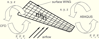
To understand the communication between the MpCCI coupling server, ABAQUS, and the third-party analysis software, consider the following high-level description of the fluid-structure interaction example problem illustrated in Figure 13.1.3–1.
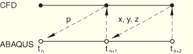
Airflow over an airplane wing builds up a pressure distribution, which causes the wing to deform. The deformation causes the airflow to change, which in turn causes the pressure distribution to vary. Given the airflow and current geometry of the wing, the computational fluid dynamics CFD analysis software computes the forces exerted on the wing. ABAQUS uses these forces to compute the corresponding deformation of the wing and updates the geometry. The CFD analysis software uses the updated geometry to recompute forces exerted on the wing, and so on. For this example a serial, or Gauss-Seidel, coupling scheme is used, with the CFD analysis being the simulation leader (see Figure 13.1.3–2).The MpCCI coupling server is started and waits to hear from the clients (ABAQUS and the CFD analysis).
The clients are started, and each client establishes a connection with the MpCCI coupling server.
The MpCCI coupling server requests that each client send interface mesh definitions (topology information).
The clients send their interface mesh definitions to the MpCCI coupling server.
The MpCCI coupling server performs neighborhood searches and forms mappings between the domain interface. The relationship between the fluid cells adjacent to the wetted surface and the elements forming the wetted surface remains the same throughout the simulation. It is assumed that the fluid “sticks” on the wetted surface.
The MpCCI coupling server instructs the CFD analysis to advance to a target time and to send the pressure distribution.
The CFD analysis advances to the target time, computes a pressure distribution, and sends the pressure distribution to the MpCCI coupling server.
The MpCCI coupling server maps the pressure distribution from the CFD mesh to the ABAQUS mesh and sends the mapped pressure distribution to ABAQUS.
The MpCCI coupling server instructs ABAQUS to receive the pressure distribution and to proceed to the target time so that it can compute and send the updated geometry.
ABAQUS proceeds to the target time, updates the geometry, and sends the updated geometry to the MpCCI coupling server.
The MpCCI coupling server maps the updated geometry from the ABAQUS mesh to the CFD mesh and sends the mapped geometry to the CFD analysis.
The MpCCI coupling server instructs the CFD analysis to proceed to the target time of the next coupling step.
Steps 7–12 are repeated until the coupled simulation is completed.
The recommended procedure for solving coupled simulations is to use the MpCCI GUI to interconnect the ABAQUS model with the third-party analysis model and to start the coupled simulation. This section provides a brief overview of the MpCCI GUI and is intended to provide you with a sense of the functionality that the MpCCI GUI provides. For additional details on the MpCCI GUI or for details on how to execute a coupled analysis without using the MpCCI GUI, consult the MpCCI Technical Reference Manual. The descriptions and figures that follow are based on the version of MpCCI, Version 3.0.4, available at the time of publication of this manual; later versions of MpCCI may vary from the description here.
The MpCCI GUI guides you through a number of steps to
select the analysis software and the respective model (input) files;
define the interface region and the solution quantities that are exchanged;
optionally, specify MpCCI control parameters; and
start the coupled simulation.
The ABAQUS model and the model for the third-party analysis software must reside in separate directories referred to as the application work directory (e.g., ABAQUS work directory). This ensures that files created during the analysis by the applications do not overwrite one another.
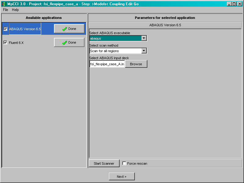
In the Models panel, shown in Figure 13.1.3–3, you select the analysis software (referred to as “applications” in the MpCCI GUI) that will participate in the coupled simulation. For each analysis application you select the model file and provide application-specific parameters (such as version numbers, etc.). If the analysis is on a remote platform, you can specify the host name and directory in the Open File dialog box. For each application you will scan the application model files to extract analysis information required for subsequent input to the MpCCI GUI.
After defining the models and scanning the input files, click Next to advance to the Coupling panel.
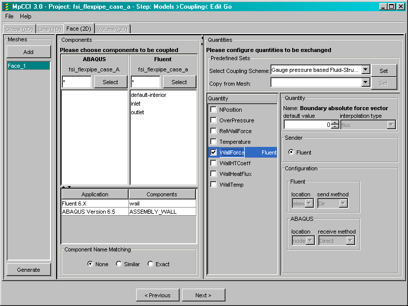
As described in “Preparing an ABAQUS analysis for co-simulation,” Section 13.1.2, you must identify the interface and the solution quantities being transferred across the interface by using the Coupling panel of the GUI, shown in Figure 13.1.3–4. In MpCCI terminology, interface “mesh” refers to interface regions and a “component” refers to, for example, surfaces in ABAQUS and wall zones in FLUENT. A mesh consists of one or more components from each analysis. For each mesh you can specify the solution quantities that are transferred.
After completing the coupling definition, click Next to advance to the Edit panel.
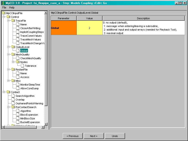
In the Edit panel, shown in Figure 13.1.3–5, you can modify any of the default MpCCI settings. These settings control the search algorithms, solution mapping schemes, and behavior of the MpCCI server. For further details, see the MpCCI Technical Reference Manual.
After modifying the MpCCI settings, click Next to advance to the Go panel.
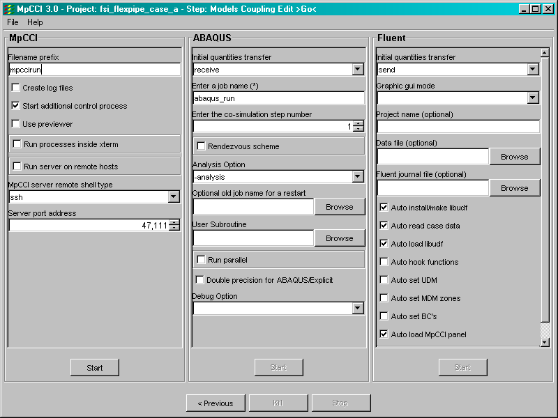
In the Go panel, shown in Figure 13.1.3–6, you can provide specific information about starting the analysis software; in the case of ABAQUS you can set the number of processors, specify user subroutines, and other parameters. Most of these settings are available for convenience in the MpCCI GUI; alternatively, you can specify these settings in the ABAQUS environment file (see “Using the ABAQUS environment settings,” Section 3.3.1).
Start the MpCCI coupling server and the third-party analysis software from the MpCCI GUI by clicking Start. You can monitor the ABAQUS job by inspecting the message file, which will include messages identifying the increments at which coupling occurs, as well as by reviewing the results in the Visualization module of ABAQUS/CAE.
ABAQUS job execution will occur in the directory where the ABAQUS input file is located. Job parameters not set in the GUI will be determined according to normal ABAQUS conventions (see “Execution procedure for ABAQUS/Standard and ABAQUS/Explicit,” Section 3.2.2).
During a co-simulation step ABAQUS suspends operations periodically at one of two locations, referred to as synchronization points, in the analysis and performs a data exchange with the third-party software. The first synchronization point is located at the start of the co-simulation analysis step, prior to commencing the first increment. This synchronization point will be called only once and, hence, allows for initial loads to be imported into ABAQUS and for the current geometry and/or temperature to be exported. The second synchronization point occurs at the end of a completed increment when the target time is reached in ABAQUS. This synchronization point is called multiple times as the simulation advances in time. At every synchronization point ABAQUS waits to receive the requested data from the third-party analysis software before continuing. Therefore, for a two-way coupled simulation the synchronization point represents a point when both analyses coincide in solution time.
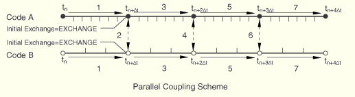
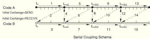
MpCCI enables you to choose one of two basic coupling schemes. Figure 13.1.3–7 and Figure 13.1.3–8 illustrate the parallel (Jacobi) and serial (Gauss-Seidel) coupling schemes that are available. The horizontal lines represent simulation time. The vertical lines represent increments (or time steps) for a particular analysis in the coupled simulation. The dashed arrows denote data exchange in the direction of the arrowheads between the analysis codes.
The coupling scheme is defined by setting the initial exchange variable in the MpCCI GUI Go panel for each analysis software. The variable can be set to values of SEND, RECEIVE, or EXCHANGE. These values define whether the analysis codes will send, receive, or exchange (send and receive) data at the first synchronization point and, thus, determines the coupling scheme as defined in Table 13.1.3–1.
Table 13.1.3–1 Coupling schemes defined by the initial exchange variable.
| Code A | ||||
| Code B | SEND | RECEIVE | EXCHANGE | |
| SEND | — | Serial | Parallel | |
| RECEIVE | Serial | — | Parallel | |
| EXCHANGE | Parallel | Parallel | Parallel | |
No data exchange occurs when the step time has been reached.
In the serial coupling scheme (also known as the Gauss-Seidel, “ping-pong,” or tandem coupling scheme) one code runs to a predetermined target time, while the other code waits. At the rendezvous or target time the solution variables are passed to the other code, which then advances to the target time, while the partner code waits. This sequence of steps completes a coupling step, at the end of which the solution quantities are up to date. As illustrated in Figure 13.1.3–8, code A, the simulation leader, advances to the first target time while code B waits. At the target time, code A sends its solution quantities to code B. Code B uses these solution quantities to advance to the target time, while code A waits. When code B reaches the target time, it sends it solution quantities to code A. This completes a coupling step; this sequence of steps is repeated for the entire simulation.
In the parallel coupling scheme both analysis codes run concurrently, exchanging solution quantities from the previous exchange to update the solution at the next coupling step. As illustrated in Figure 13.1.3–7, both analysis codes advance (arrow 1) with loads and/or boundary conditions exchanged at the initial synchronization point. At the second synchronization point the analysis codes exchange solution quantities (arrow 2). Only when the exchange has been completed—both the send and receive transactions have completed—will each code proceed to the next coupling step (represented by the arrows labeled 3 and 4). Thus, there is a lag in the loads received and the solution quantities computed by one coupling step. This lag is typical for a parallel algorithm and may lead to solution accuracy issues.
When deciding on the coupling scheme, you should consider solution accuracy as well as the utilization impact on your computing resources. The serial coupling scheme can lead to inefficient use of computing resources in cases where the simulations are run on separate machines. In these situations a parallel coupling scheme may make more efficient use of resources. In other cases where the two simulations are run on the same machine, it may be more efficient to employ the serial scheme, allowing each simulation complete use of the machine resources.
Different types of analyses have different time incrementation requirements, which will influence or dictate the frequency of interaction between ABAQUS and the third-party analysis software to obtain an accurate and robust solution.
For example, consider the difference in time incrementation between an implicit and an explicit dynamic analysis. Another example is a transient heat transfer analysis modeling a diffusive process; here the analysis may use small time increments at the beginning of the analysis where there is a high gradient in the solution and large time increments toward the end of the analysis when steady state is achieved. In this case ABAQUS can automatically adjust the increment sizes to obtain an economical and accurate solution.
To be flexible to accommodate different third-party analysis software, ABAQUS offers several rendezvousing schemes that define the exchange frequency between ABAQUS and the third-party software. In each scheme the target times in ABAQUS can be reached in an exact or loose manner, as discussed in “Exact versus loose coupling,” below. The rendezvousing schemes are defined through the MpCCI GUI Go panel and are discussed in the following sections.
This rendezvousing scheme assumes that both analyses advance and exchange data according to
![]()
In the Go panel of the MpCCI GUI, select the rendezvousing scheme and specify the coupling step size used by ABAQUS. It is your responsibility to ensure that the coupling step size used by ABAQUS and the third-party analysis software match for a transient simulation. No checks are performed by MpCCI to ensure this condition.
Each step in an ABAQUS analysis is divided into multiple increments, and in most cases you have two choices for controlling the solution: automatic time incrementation or direct user-specified time incrementation. This rendezvousing scheme can be employed with either method. When used with direct time incrementation, you can choose the time increment size to match the coupling step size. In this case both the ABAQUS analysis and the third-party analysis are advanced, and data are exchanged at a constant step size. Alternatively, you can allow ABAQUS to subcycle; that is, to take two or more time increments before the target time is reached. In this case you select the coupling step size to be a multiple of the increment size used in ABAQUS. When used with automatic time incrementation, ABAQUS allows for adjustments in the increment size while ensuring that the exchange occurs at a regular enough frequency for solution stability.
When selecting this rendezvousing scheme, ABAQUS dictates the coupling step size to the third-party software. This scheme allows for a time varying coupling step size that is adjusted based on the ABAQUS solution. In this case the third-party software must be able to adjust the coupling step time to use ABAQUS's suggested value.
The suggested coupling step size is computed at the end of the previous coupling step and remains constant during the current coupling step. If automatic time incrementation is selected, ABAQUS may cut back and use multiple increments to meet the target time.
When selecting this rendezvousing scheme, ABAQUS receives a coupling step size from the third-party analysis software to compute the target time. This scheme allows for a time varying coupling step size that is adjusted based on the solution of the third-party application. ABAQUS may take one or more increments to reach the target time.
A special case of a coupled simulation is a steady-state analysis. In this case time is not physically meaningful and is used as a parameter to measure the forward progress in a steady-state solution without regard to the true transient behavior. For steady-state problems the coupling time reflects only the computational step at which data are transferred; thus, the demands on the coupling algorithm may be relaxed. Any of the rendezvousing schemes discussed can be used for steady-state simulations.
To use the asynchronous or on-demand method, use direct time incrementation for the ABAQUS procedure. Adjust the time increment and total time such that sufficient exchanges can be performed. For example, if you want to have 10 exchanges, you can set the time increment equal to 1.0 and the total time equal to 10. Every time an exchange is requested, ABAQUS advances the time increment by one. The simulation can be stopped from the MpCCI GUI in case a steady-state solution is reached prior to the total time by using the STOP button. In this case ABAQUS terminates the analysis.
To reach the target time, ABAQUS may perform several increments. These increments are referred to as “subcycling.” ABAQUS/Standard ramps loads (with the exception of film properties) from the values of the previous coupling step to the values at the target time. In ABAQUS/Explicit the loads are applied at the start of the coupling step and kept constant over the coupling step.
In ABAQUS the target times can be reached in an exact or loose manner. By default, ABAQUS exchanges the data in an exact manner; that is, ABAQUS temporarily reduces the time increment so that the solution exchange occurs exactly at the target time. With the loose coupling method, the solution exchange occurs when the current simulation time, t, is within half of a coupling step size away from the target exchange time,
![]()
For accuracy considerations, loose coupling should be employed only for cases where ABAQUS uses more increments than the third-party analysis software during a coupling step.
Global convergence of a coupled simulation is assumed when the individual analyses have converged to their specified tolerances, referred to as local convergence. Local convergence for nonlinear ABAQUS/Standard problems is discussed in “Solving nonlinear problems,” Section 7.1.1. These ABAQUS/Standard criteria are unaffected by the co-simulation interaction with third-party software and will be met before the coupled simulation will proceed to the next coupling step in ABAQUS.
The coupling schemes provided are globally explicit; that is, the loads and boundary conditions for the next coupling step are determined based on the solution of the previous coupling step. Hence, the overall convergence of a coupled solution is expected to behave similarly to that of an explicit algorithm; transient problems will require a suitable rendezvousing scheme such that data are exchanged with a frequency that ensures overall solution stability.
Interface loads imported into ABAQUS are not saved to the ABAQUS restart database. Thus, to restart a co-simulation, the third-party analysis software has to send the loads at the start of the restart analysis. These loads from the CFD analysis have to balance the current deformation of the ABAQUS analysis such that the structure is in equilibrium. It is your responsibility to synchronize the restart information written between the analyses. Furthermore, you must ensure that the simulation is restarted at the same solution (step) time. For example, to restart an FSI co-simulation, the solution time for the particular step/increment number from which ABAQUS is restarted has to correspond to the CFD solution.
The following software is required:
MpCCI Version 3.0.5. MpCCI is distributed and licensed by Fraunhofer SCAI. For contact information, refer to http://www.scai.fraunhofer.de.