Products: ABAQUS/Standard ABAQUS/CAE
Solving nonlinear problems in ABAQUS/Standard involves:
a combination of incremental and iterative procedures;
using the Newton method to solve the nonlinear equations;
determining convergence;
defining loads as a function of time; and
choosing suitable time increments automatically.
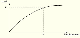
The nonlinear load-displacement curve for a structure is shown in Figure 7.1.1–1.
The objective of the analysis is to determine this response. In a nonlinear analysis the solution cannot be calculated by solving a single system of linear equations, as would be done in a linear problem. Instead, the solution is found by specifying the loading as a function of time and incrementing time to obtain the nonlinear response. Therefore, ABAQUS/Standard breaks the simulation into a number of time increments and finds the approximate equilibrium configuration at the end of each time increment. Using the Newton method, it often takes ABAQUS/Standard several iterations to determine an acceptable solution to each time increment.The time history for a simulation consists of one or more steps. You define the steps, which generally consist of an analysis procedure, loading, and output requests. Different loads, boundary conditions, analysis procedures, and output requests can be used in each step. For example:
Step 1: Hold a plate between rigid jaws.
Step 2: Add loads to deform the plate.
Step 3: Find the natural frequencies of the deformed plate.
An increment is part of a step. In nonlinear analyses each step is broken into increments so that the nonlinear solution path can be followed. You suggest the size of the first increment, and ABAQUS/Standard automatically chooses the size of the subsequent increments. At the end of each increment the structure is in (approximate) equilibrium and results are available for writing to the restart, data, results, or output database files.
An iteration is an attempt at finding an equilibrium solution in an increment. If the model is not in equilibrium at the end of the iteration, ABAQUS/Standard tries another iteration. With every iteration the solution that ABAQUS/Standard obtains should be closer to equilibrium; however, sometimes the iteration process may diverge—subsequent iterations may move away from the equilibrium state. In that case ABAQUS/Standard may terminate the iteration process and attempt to find a solution with a smaller increment size.
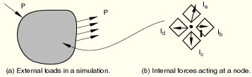
Consider the external forces, P, and the internal (nodal) forces, I, acting on a body (see Figure 7.1.1–2(a) and Figure 7.1.1–2(b), respectively). The internal loads acting on a node are caused by the stresses in the elements that are attached to that node.
For the body to be in equilibrium, the net force acting at every node must be zero. Therefore, the basic statement of equilibrium is that the internal forces, I, and the external forces, P, must balance each other:
![]()
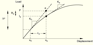
The nonlinear response of a structure to a small load increment, ![]() , is shown in Figure 7.1.1–3. ABAQUS/Standard uses the structure's tangent stiffness,
, is shown in Figure 7.1.1–3. ABAQUS/Standard uses the structure's tangent stiffness, ![]() , which is based on its configuration at
, which is based on its configuration at ![]() , and
, and ![]() to calculate a displacement correction,
to calculate a displacement correction, ![]() , for the structure. Using
, for the structure. Using ![]() , the structure's configuration is updated to
, the structure's configuration is updated to ![]() .
.
ABAQUS/Standard then calculates the structure's internal forces, ![]() , in this updated configuration. The difference between the total applied load, P, and
, in this updated configuration. The difference between the total applied load, P, and ![]() can now be calculated as
can now be calculated as
![]()
If ![]() is zero at every degree of freedom in the model, point a in Figure 7.1.1–3 would lie on the load-deflection curve and the structure would be in equilibrium. In a nonlinear problem
is zero at every degree of freedom in the model, point a in Figure 7.1.1–3 would lie on the load-deflection curve and the structure would be in equilibrium. In a nonlinear problem ![]() will never be exactly zero, so ABAQUS/Standard compares it to a tolerance value. If
will never be exactly zero, so ABAQUS/Standard compares it to a tolerance value. If ![]() is less than this force residual tolerance at all nodes, ABAQUS/Standard accepts the solution as being in equilibrium. By default, this tolerance value is set to 0.5% of an average force in the structure, averaged over time. ABAQUS/Standard automatically calculates this spatially and time-averaged force throughout the simulation. You can change this, and all other such tolerances, by specifying solution controls (see “Convergence criteria for nonlinear problems,” Section 7.2.3).
is less than this force residual tolerance at all nodes, ABAQUS/Standard accepts the solution as being in equilibrium. By default, this tolerance value is set to 0.5% of an average force in the structure, averaged over time. ABAQUS/Standard automatically calculates this spatially and time-averaged force throughout the simulation. You can change this, and all other such tolerances, by specifying solution controls (see “Convergence criteria for nonlinear problems,” Section 7.2.3).
If ![]() is less than the current tolerance value, P and
is less than the current tolerance value, P and ![]() are considered to be in equilibrium and
are considered to be in equilibrium and ![]() is a valid equilibrium configuration for the structure under the applied load. However, before ABAQUS/Standard accepts the solution, it also checks that the last displacement correction,
is a valid equilibrium configuration for the structure under the applied load. However, before ABAQUS/Standard accepts the solution, it also checks that the last displacement correction, ![]() , is small relative to the total incremental displacement,
, is small relative to the total incremental displacement, ![]() . If
. If ![]() is greater than a fraction (1% by default) of the incremental displacement, ABAQUS/Standard performs another iteration. Both convergence checks must be satisfied before a solution is said to have converged for that time increment.
is greater than a fraction (1% by default) of the incremental displacement, ABAQUS/Standard performs another iteration. Both convergence checks must be satisfied before a solution is said to have converged for that time increment.
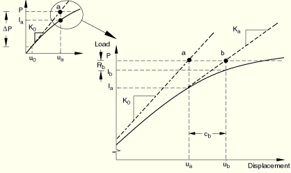
If the solution from an iteration is not converged, ABAQUS/Standard performs another iteration to try to bring the internal and external forces into balance. First, ABAQUS/Standard forms the new stiffness, ![]() , for the structure based on the updated configuration,
, for the structure based on the updated configuration, ![]() . This stiffness, together with the residual
. This stiffness, together with the residual ![]() , determines another displacement correction,
, determines another displacement correction, ![]() , that brings the system closer to equilibrium (point b in Figure 7.1.1–4).
, that brings the system closer to equilibrium (point b in Figure 7.1.1–4).
ABAQUS/Standard calculates a new force residual, ![]() , using the internal forces from the structure's new configuration,
, using the internal forces from the structure's new configuration, ![]() . Again, the largest force residual at any degree of freedom,
. Again, the largest force residual at any degree of freedom, ![]() , is compared against the force residual tolerance, and the displacement correction for the second iteration,
, is compared against the force residual tolerance, and the displacement correction for the second iteration, ![]() , is compared to the increment of displacement,
, is compared to the increment of displacement, ![]() . If necessary, ABAQUS/Standard performs further iterations. For more details on convergence in ABAQUS/Standard, see “Convergence criteria for nonlinear problems,” Section 7.2.3.
. If necessary, ABAQUS/Standard performs further iterations. For more details on convergence in ABAQUS/Standard, see “Convergence criteria for nonlinear problems,” Section 7.2.3.
For each iteration in a nonlinear analysis ABAQUS/Standard forms the model's stiffness matrix and solves a system of equations. Therefore, the computational cost of each iteration is close to the cost of conducting a complete linear analysis, making the computational expense of a nonlinear analysis potentially many times greater than the cost of a linear analysis. Since it is possible with ABAQUS/Standard to save results at each converged increment, the amount of output data available from a nonlinear simulation can also be much greater than that available from a linear analysis of the same geometry.
By default, ABAQUS/Standard automatically adjusts the size of the time increments to solve nonlinear problems efficiently. You need to suggest only the size of the first increment in each step of the simulation, after which ABAQUS/Standard automatically adjusts the size of the increments. If you do not provide a suggested initial increment size, ABAQUS/Standard will attempt to apply all of the loads defined in the step in a single increment. For highly nonlinear problems ABAQUS/Standard will have to reduce the increment size repeatedly to obtain a solution, resulting in wasted CPU time. It is advantageous to provide a reasonable initial increment size because only in mildly nonlinear problems can all of the loads in a step be applied in a single increment.
The number of iterations needed to find a converged solution for a time increment will vary depending on the degree of nonlinearity in the system. With the default incrementation control, the procedure works as follows. If the solution has not converged within 16 iterations or if the solution appears to diverge, ABAQUS/Standard abandons the increment and starts again with the increment size set to 25% of its previous value. It then attempts to find a converged solution with this smaller time increment. If the solution still fails to converge, ABAQUS/Standard reduces the increment size again. This process is continued until a solution is found. If the time increment becomes smaller than the minimum you defined or more than 5 attempts are needed, ABAQUS/Standard stops the analysis.
If the increment converges in fewer than 5 iterations, this indicates that the solution is being found fairly easily. Therefore, ABAQUS/Standard automatically increases the increment size by 50% if 2 consecutive increments require fewer than 5 iterations to obtain a converged solution.
While the default automatic incrementation control is suitable for most analyses, you can change all the defaults when necessary by specifying solution controls; see “Commonly used control parameters,” Section 7.2.2, and “Time integration accuracy in transient problems,” Section 7.2.4.
Nonlinear static problems can be unstable. Such instabilities may be of a geometrical nature, such as buckling, or of a material nature, such as material softening. If the instability manifests itself in a global load-displacement response with a negative stiffness, the problem can be treated as a buckling or collapse problem as described in “Unstable collapse and postbuckling analysis,” Section 6.2.4. However, if the instability is localized, there will be a local transfer of strain energy from one part of the model to neighboring parts, and global solution methods may not work. This class of problems has to be solved either dynamically or with the aid of (artificial) damping; for example, by using dashpots.
ABAQUS/Standard provides an automatic mechanism for stabilizing unstable quasi-static problems through the automatic addition of volume-proportional damping to the model. The mechanism is triggered by including automatic stabilization in any nonlinear quasi-static procedure. Viscous forces of the form
![]()
![]()
For the case of static stabilization the mass matrix for Timoshenko beams is always calculated assuming isotropic rotary inertia, regardless of the type of rotary inertia specified for the beam section definition (“Rotary inertia for Timoshenko beams” in “Beam section behavior,” Section 23.3.5).
Automatic stabilization does not carry over automatically to subsequent steps. It needs to be declared for any step in which you want it to be active. ABAQUS/Standard recalculates new values for the damping factor, based on the declared damping intensity and on the solution of the first increment of the step. Therefore, unless you specify the same damping factor directly (see “Using the damping factor” below), an analysis with an unstable step may produce slightly different results from the same analysis with the original step split into two steps. Moreover, if the instabilities in the model have not subsided by the end of a step, viscous forces may be terminated abruptly or modified at the beginning of subsequent steps, potentially causing convergence difficulties if automatic stabilization is not used in the subsequent step. If such a situation arises, it is recommended that the problem be restarted with the damping factor set equal to the value chosen by ABAQUS/Standard (or to the value you specified) in the previous step. This value is printed in the message (.msg) file for the previous step. If it is necessary to have an accurate static equilibrium solution after an instability has occurred (and the model's behavior has returned to a stable regime), the step with automatic stabilization can be followed by a step without such stabilization.
It is assumed that the problem is stable at the beginning of the step and that instabilities may develop in the course of the step. While the model is stable, viscous forces and, therefore, the viscous energy dissipated are very small. Thus, the additional artificial damping has no effect. If a local region goes unstable, the local velocities increase and, consequently, part of the strain energy then released is dissipated by the applied damping. ABAQUS/Standard can, if necessary, reduce the time increment to permit the process to occur without the unstable response causing very large displacements. ABAQUS/Standard calculates and prints to the message file the damping factor, c, based on the solution of the first increment of a step. In most applications the first increment of the step is stable without the need to apply damping. The damping factor is then determined in such a way that the extrapolated dissipated energy for the step is a small fraction of the extrapolated strain energy. The fraction is called the dissipated energy fraction and has a default value of 2.0 × 10⁻⁴.
Alternatively, you can specify the dissipated energy fraction for automatic stabilization directly.
| Input File Usage: | Use any of the following options to activate automatic stabilization with the default dissipated energy fraction: |
*COUPLED TEMPERATURE-DISPLACEMENT, STABILIZE
*SOILS, STABILIZE
*STATIC, STABILIZE
*STEADY STATE TRANSPORT, STABILIZE
*VISCO, STABILIZE
Use any of the following options to specify a nondefault dissipated energy fraction: *COUPLED TEMPERATURE-DISPLACEMENT, STABILIZE=dissipated energy fraction *SOILS, STABILIZE=dissipated energy fraction *STATIC, STABILIZE=dissipated energy fraction *STEADY STATE TRANSPORT, STABILIZE=dissipated energy fraction *VISCO, STABILIZE=dissipated energy fraction |
| ABAQUS/CAE Usage: | Step module: Create Step: General: any valid step type: Basic: toggle on Use stabilization with, and select dissipated energy fraction |
The procedure of computing an appropriate damping factor works well for many applications. However, there are cases where the computed damping factor is either too small, thus not controlling the instability, or too high, thus leading to inaccurate results. This occurs when a poor estimation of the extrapolated strain energy is made during the first increment. For example, consider a sequentially coupled thermal-stress analysis in which a mechanical analysis reads temperatures from a previous transient thermal analysis. Typically the thermal analysis exhibits a diffusive process, where rapid changes in temperature occurs early in the analysis and minor changes in temperature occur once steady state is reached. In such a case ABAQUS will compute the extrapolated strain energy based on the temperatures corresponding to the time of the first increment (in this case there may be a significant change in temperature for the first increment), thus yielding a larger then expected extrapolated strain energy. This in turn leads to a damping factor that is too large, resulting in inaccurate results.
With automatic stabilization, check the following to ensure that accurate solutions are obtained:
Check the damping factor printed to the message (.msg) file at the end of the first increment to ensure that a reasonable amount of damping is applied. Unfortunately, the damping factor is problem dependent; therefore, you must rely on experience from previous runs.
Compare the viscous forces (VF) with the overall forces in the analysis, and ensure that the viscous forces are relatively small compared with the overall forces in the model.
Compare the viscous damping energy (ALLSD) with the total strain energy (ALLSE), and ensure that the ratio does not exceed the dissipated energy fraction or any reasonable amount. The viscous damping energy may be large if the structure undergoes a large amount of motion.
There are cases where the first increment is either unstable or singular (due to a rigid body mode). In such cases it is not possible to obtain a solution to the first increment without applying some damping. Therefore, some damping is already applied during the first increment. The damping factor used for the initial increment is chosen such that the average element damping matrix component, divided by the step time, is equal to the average element stiffness matrix component multiplied by the dissipated energy fraction. If the calculated strain energy change in this increment indicates that the solution without damping is stable, the damping factor is recalculated based upon the energy method described in the previous paragraph. However, if the strain energy change indicates that the solution is unstable or singular, the initially calculated damping factor is maintained, and a warning message is issued indicating that the amount of damping applied may not be appropriate. In many cases the amount of damping may actually be rather large, which can affect the solution in ways that are not desirable. Therefore, if the above mentioned warning message is issued, check the viscous forces (VF) and compare them with the expected nodal forces to make sure that the viscous forces do not dominate the solution. If necessary, follow the stabilized step with another step in which stabilization is not used or with a step in which a much smaller damping factor is used.
Alternatively, you can specify the damping factor directly. Unfortunately, it is quite difficult to make a reasonable estimate for the damping factor, unless a value is known from the output of previous runs; the damping factor includes information not only about the amount of damping but also about mesh size and material behavior.
| Input File Usage: | Use any of the following options to specify the damping factor directly: |
*COUPLED TEMPERATURE-DISPLACEMENT, STABILIZE, FACTOR=damping factor *SOILS, STABILIZE, FACTOR=damping factor *STATIC, STABILIZE, FACTOR=damping factor *STEADY STATE TRANSPORT, STABILIZE, FACTOR=damping factor *VISCO, STABILIZE, FACTOR=damping factor |
| ABAQUS/CAE Usage: | Step module: Create Step: General: Coupled temp-displacement, Soils, Static, General, or Visco: Basic: toggle on Use stabilization with, and select damping factor |