Products: ABAQUS/Standard ABAQUS/CAE
A random response analysis:
is a linear perturbation procedure that gives the linearized dynamic response of a model to user-defined random excitation; and
uses the set of modes extracted in a previous eigenfrequency extraction step to calculate the power spectral densities of response variables (stresses, strains, displacements, etc.) and the corresponding root mean square (RMS) values of these same variables.
Random response analysis predicts the response of a system that is subjected to a nondeterministic continuous excitation that is expressed in a statistical sense by a cross-spectral density matrix. Since the loading is nondeterministic, it can be characterized only in a statistical sense; ABAQUS/Standard assumes that the excitation is stationary and ergodic. These statistical measures are explained in detail in “Random response analysis,” Section 2.5.8 of the ABAQUS Theory Manual. The random response procedure can, for example, be used to determine the response of an airplane to turbulence, the response of a car to road surface imperfections, the response of a structure to jet noise, or the response of a building to an earthquake.
In the most general case the excitation is defined as a frequency-dependent cross-spectral density (CSD) matrix. Except in cases involving moving noise or user subroutine UCORR, it is assumed that for a given load case the CSD matrix can be separated into a product of a frequency-dependent, complex-valued scalar function and a frequency-independent, complex-valued, spatial correlation matrix. This assumption helps reduce both the computational time and the amount of required user input but implies that each element of the CSD matrix in a given load case has the same frequency dependence. You can define a different frequency dependence for each load case, but the loads in one load case will not be correlated with loads in another. Consequently, the system CSD matrix is assembled by simply summing (superimposing) the CSD matrices of the individual load cases.
The frequency-dependent scalar function can be composed of a weighted sum of user-defined, complex-valued, frequency functions. These user-defined frequency functions are specified in units of power spectral density. You assign weights to each frequency function as well as specify properties of the spatial correlation matrix that defines the correlation between excitations at different locations and in different directions for a particular load case. Frequency functions and correlations are discussed below; see “Defining the frequency functions,” and “Defining the correlation.”
The loads can be defined as concentrated point loads, as distributed loads, as connector element loads, or as base motion excitations, as described below in “Boundary conditions,” and “Loads.” Multiple, uncorrelated load cases can be defined for concentrated point loads, connector loads, and base motions. Load case 1 is reserved for all distributed loads defined in a particular step. In these steps load case 1 cannot be used for any concentrated point load, connector load, or base motion. Thus, there cannot be any correlation between distributed loads and any other load. Moreover, base motion excitations are assumed to be statistically independent (no correlation) with any other load type even when the same load case number is used. The concentrated point and connector element loads are assumed to be correlated if the same load case number is used.
The random response procedure is based on using a subset of the modes of the system, which must first be extracted by using the eigenfrequency extraction procedure. The modes will include eigenmodes and, if activated in the eigenfrequency extraction step, residual modes. The number of modes extracted must be sufficient to model the dynamic response of the system adequately, which is a matter of judgment on your part. The model can be preloaded prior to the eigenfrequency extraction. Initial stress effects are included in the stiffness used in the eigenfrequency extraction if geometric nonlinearities are included in the general analysis procedure used to apply the preloads (“General and linear perturbation procedures,” Section 6.1.2).
The random response of the model is expressed as power spectral density values of nodal and element variables, as well as their root mean square values.
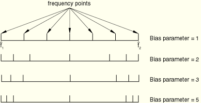
You specify the frequency range of interest for the random response procedure. The response is calculated at multiple points between the lowest frequency of interest and the first eigenfrequency in the range, between each eigenfrequency in the range, and between the last eigenfrequency in the range and the highest frequency in the range as illustrated in Figure 6.3.11–1. The default number of calculation points in each interval is 20; you can change this number when you define the step. Accurate RMS values can be obtained only if enough points are used so that ABAQUS/Standard can integrate accurately over the frequency range. The bias function allows the points on the frequency scale to be spaced closer together at the eigenfrequencies, thus allowing detailed definition of the response close to resonant frequencies and more accurate integration.
| Input File Usage: | *RANDOM RESPONSE lower_freq_limit, upper_freq_limit, num_calc_pts, bias_parameter, freq_scale |
| ABAQUS/CAE Usage: | Step module: Create Step: Linear perturbation: Random response |
The bias parameter can be used to provide closer spacing of the result points either toward the middle or toward the ends of each frequency interval. Figure 6.3.11–2 shows a few examples of the effect of the bias parameter on the frequency spacing.
The bias formula used to calculate the frequency at which results are presented is as follows:
![]()
y
![]() ;
;
n
is the number of frequency points at which results are to be given;
k
is one such frequency point (![]() );
);
![]()
is the lower limit of the frequency interval;
![]()
is the upper limit of the interval;
![]()
is the frequency at which the kth results are given;
p
is the bias parameter value; and
![]()
is the frequency or the logarithm of the frequency, depending on the chosen frequency scale.
To define the random loading, you specify a frequency function and a cross-correlation definition that refers to the frequency function. The frequency functions are defined as model data (i.e., they are step independent) and must be named. A log-log scale is used in interpolating between the given values.
The type of units in the CSD matrix of the excitation are specified as part of the frequency function definition. The default type is power units. If the CSD matrix of the excitation is due to base motion, the units must be in g units and you should define the acceleration of gravity. Alternatively, decibel units can be specified; this type of units is explained below.
| Input File Usage: | Use one of the following options to define the frequency function: |
*PSD-DEFINITION, NAME=name, TYPE=FORCE (default; power units) *PSD-DEFINITION, NAME=name, TYPE=BASE, G=g *PSD-DEFINITION, NAME=name, TYPE=DB, DB REFERENCE= |
| ABAQUS/CAE Usage: | You cannot define a frequency function in ABAQUS/CAE. |
In ABAQUS/Standard the decibel value ![]() is related to the frequency function
is related to the frequency function ![]() by the following full octave band conversion formula:
by the following full octave band conversion formula:
![]()
Table 6.3.11–1 Standard octave bands.
| Band number | Band center (frequency, Hz) |
|---|---|
| 1 | 1.0 |
| 2 | 2.0 |
| 3 | 4.0 |
| 4 | 8.0 |
| 5 | 16.0 |
| 6 | 31.5 |
| 7 | 63.0 |
| 8 | 125.0 |
| 9 | 250.0 |
| 10 | 500.0 |
| 11 | 1000.0 |
| 12 | 2000.0 |
| 13 | 4000.0 |
| 14 | 8000.0 |
| 15 | 16000.0 |
![]()
![]() in decibels must be specified as a function of the frequency band; the associated midband frequencies are given in Table 6.3.11–1.
in decibels must be specified as a function of the frequency band; the associated midband frequencies are given in Table 6.3.11–1.
You can define a frequency function in an external file or in a user subroutine.
The data to define a frequency function can be contained in an external file.
| Input File Usage: | *PSD-DEFINITION, NAME=name, TYPE=type, INPUT=file name |
| ABAQUS/CAE Usage: | You cannot define a frequency function in ABAQUS/CAE. |
Complicated frequency functions can be more easily defined by user subroutine UPSD than by entering data directly.
| Input File Usage: | *PSD-DEFINITION, NAME=name, TYPE=type, USER |
Any data lines given will be ignored if the USER parameter is specified. |
| ABAQUS/CAE Usage: | User subroutine UPSD is not supported in ABAQUS/CAE. |
You define the cross-correlation between the applied nodal loads or base motions. You can also assign scaling (weight) factors to the frequency functions through the cross-correlation definition. Distributed loads are converted to equivalent nodal loads, which are treated as individual point loads with respect to the cross-correlation. The cross-correlation is defined in the random response step and references a particular load case number and frequency function.
Three types of correlation can be defined: correlated, uncorrelated, and moving noise. As many correlations as needed to define the random loading can be specified unless the moving noise type is chosen, in which case only one correlation can appear in the step definition.
For the correlated type all terms in the cross-spectral density matrix are considered, which implies that the loads on all degrees of freedom within the load case are fully correlated (statistically dependent on each other).
For the uncorrelated type only diagonal terms in the cross-spectral density matrix are considered, which implies that no correlation exists between the load on one degree of freedom and the load on another. You should exercise caution when choosing the uncorrelated type with distributed loads since the equivalent nodal forces would be uncorrelated with each other (statistically independent).
For the moving noise type the terms in the correlation matrix depend on the relative position of the points where the loads are applied. This type can be used only in conjunction with concentrated point loads and distributed loads. In addition, the moving noise formulation assumes that the frequency function referenced by the cross-correlation defines a reference power spectral density function of the noise source. (It is a reference power spectral density because it can later be scaled by the magnitude of the loadings specified as distributed, concentrated point, or connector element loads.) Since the power spectral density is real-valued for real-valued variables, the frequency function must not contain imaginary terms when used with the moving noise type of cross-correlation.
| Input File Usage: | Use one of the following options to define the correlation: |
*CORRELATION, TYPE=CORRELATED, PSD=name
*CORRELATION, TYPE=UNCORRELATED, PSD=name
*CORRELATION, TYPE=MOVING NOISE
For the moving noise type the reference to the power spectral density function must be given on each data line. |
| ABAQUS/CAE Usage: | You cannot define a correlation in ABAQUS/CAE. |
For correlated or uncorrelated cross-correlations you can specify whether or not both real and imaginary terms will be included in the spatial correlation matrix. This specification does not affect the imaginary terms given for the power spectral density frequency function.
| Input File Usage: | Use one of the following options: |
*CORRELATION, TYPE=CORRELATED, COMPLEX=YES or NO, PSD=name *CORRELATION, TYPE=UNCORRELATED, COMPLEX=YES or NO, PSD=name |
| ABAQUS/CAE Usage: | You cannot define a correlation in ABAQUS/CAE. |
You can define a correlation in an external input file or in a user subroutine.
The data to define a correlation can be contained in an external input file.
| Input File Usage: | *CORRELATION, TYPE=type, PSD=name, INPUT=file_name |
| ABAQUS/CAE Usage: | You cannot define a correlation in ABAQUS/CAE. |
Simple excitations, such as uncorrelated white noise, are easily defined. Excitations involving more complicated correlations, including cases where the elements of the CSD matrix have different frequency dependencies, can be defined through user subroutine UCORR. If the user subroutine is specified, only the load case number must be entered as part of the correlation definition. A user subroutine cannot be used to define a moving noise correlation.
For uncorrelated cross-correlations only the diagonal terms of the correlation matrix specified in UCORR will be used. The combination of the cross-correlation with the various kinds of applied loads is discussed in more detail below.
| Input File Usage: | Use one of the following options: |
*CORRELATION, TYPE=CORRELATED, USER, COMPLEX=YES or NO, PSD=name *CORRELATION, TYPE=UNCORRELATED, USER, PSD=name |
| ABAQUS/CAE Usage: | User subroutine UCORR is not supported in ABAQUS/CAE. |
You can select the modes to be used in modal superposition and specify damping values for all selected modes.
You can select modes by specifying the mode numbers individually, by requesting that ABAQUS/Standard generate the mode numbers automatically, or by requesting the modes that belong to specified frequency ranges. If you do not select the modes, all modes extracted in the prior eigenfrequency extraction step, including residual modes if they were activated, are used in the modal superposition.
| Input File Usage: | Use one of the following options to select the modes by specifying mode numbers: |
*SELECT EIGENMODES, DEFINITION=MODE NUMBERS
*SELECT EIGENMODES, GENERATE, DEFINITION=MODE NUMBERS
Use the following option to select the modes by specifying a frequency range: *SELECT EIGENMODES, DEFINITION=FREQUENCY RANGE |
| ABAQUS/CAE Usage: | You cannot select the modes in ABAQUS/CAE; all modes extracted are used in the modal superposition. |
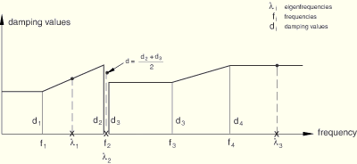
Damping is almost always specified for a random response analysis (see “Material damping,” Section 20.1.1). If damping is absent, the response of a structure will be unbounded if the forcing frequency is equal to an eigenfrequency of the structure. To get quantitatively accurate results, especially near natural frequencies, accurate specification of damping properties is essential. The various damping options available are discussed in “Material damping,” Section 20.1.1. You can define a damping coefficient for all or some of the modes used in the response calculation. The damping coefficient can be given for a specified mode number or for a specified frequency range. When damping is defined by specifying a frequency range, the damping coefficient for a mode is interpolated linearly between the specified frequencies. The frequency range can be discontinuous; the average damping value will be applied for an eigenfrequency at a discontinuity. The damping coefficients are assumed to be constant outside the range of specified frequencies.
| Input File Usage: | Use the following option to define damping by specifying mode numbers: |
*MODAL DAMPING, DEFINITION=MODE NUMBERS Use the following option to define damping by specifying a frequency range: *MODAL DAMPING, DEFINITION=FREQUENCY RANGE |
| ABAQUS/CAE Usage: | Use the following input to define damping by specifying mode numbers: |
Step module: Create Step: Linear perturbation: Random response: Damping Defining damping by specifying frequency ranges is not supported in ABAQUS/CAE. |
Figure 6.3.11–3 illustrates how the damping coefficients at different eigenfrequencies are determined for the following input:
*MODAL DAMPING, DEFINITION=FREQUENCY RANGE


The following rules apply for selecting modes and specifying modal damping coefficients:
No modal damping is included by default.
Mode selection and modal damping must be specified in the same way, using either mode numbers or a frequency range.
If you do not select any modes, all modes extracted in the prior frequency analysis, including residual modes if they were activated, will be used in the superposition.
If you do not specify damping coefficients for modes that you have selected, zero damping values will be used for these modes.
Damping is applied only to the modes that are selected.
Damping coefficients for selected modes that are beyond the specified frequency range are constant and equal to the damping coefficient specified for the first or the last frequency (depending which one is closer). This is consistent with the way ABAQUS interprets amplitude definitions.
It is not appropriate to specify initial conditions in a random response analysis.
It is not possible to prescribe nonzero displacements and rotations directly as boundary conditions (“Boundary conditions,” Section 27.3.1) in mode-based dynamic response procedures. Therefore, in a random response analysis the motion of nodes can be specified only as base motion; nonzero displacement, velocity, or acceleration history definitions given as boundary conditions are ignored, and any changes in the support conditions from the eigenfrequency extraction step are flagged as errors. In addition, any amplitude definitions are ignored in a random response analysis.
The method for prescribing motion in modal superposition procedures is described in “Transient modal dynamic analysis,” Section 6.3.7. In random response analysis only a single (primary) base can be defined.
The excitation defined by the base motion is assigned to numbered load cases. These load cases are then referenced in the cross-correlation definition. The load cases are associated with frequency functions through the reference in the cross-correlation definition. Any number of load cases can be defined, but load case number 1 cannot be used if distributed loads are defined in the same step.
| Input File Usage: | *BASE MOTION, LOAD CASE=n |
| ABAQUS/CAE Usage: | Base motions are not supported in ABAQUS/CAE. |
When the excitation is provided by a base motion, it is converted directly into a cross-spectral density matrix projected onto the eigenspace through the modal participation factors (see “Natural frequency extraction,” Section 6.3.5), giving
![]()
is the modal participation factor for mode ![]() in excitation direction i (i=1–6);
in excitation direction i (i=1–6);
![]()
is the frequency function referenced by the Jth cross-correlation and defined as a function of the frequency f in g units;
![]()
is a matrix of weight factors indicating the fraction of ![]() to be associated with the correlation between base motion in directions i and j for load case I, as described below;
to be associated with the correlation between base motion in directions i and j for load case I, as described below;
![]()
![]() , 1, or 2, depending on whether the base motion corresponding to load case I is defined in terms of an acceleration spectrum, a velocity spectrum, or a displacement spectrum (see “Transient modal dynamic analysis,” Section 6.3.7); and
, 1, or 2, depending on whether the base motion corresponding to load case I is defined in terms of an acceleration spectrum, a velocity spectrum, or a displacement spectrum (see “Transient modal dynamic analysis,” Section 6.3.7); and
![]()
is the user-specified acceleration of gravity for the same power spectral density frequency function that defines ![]() .
.
![]()
![]() for all
for all ![]() if the excitation is correlated or
if the excitation is correlated or
![]()
![]() if the excitation is uncorrelated,
if the excitation is uncorrelated,
The loading for random response analysis is defined in general terms by the cross-spectral density matrix ![]() , where f is frequency in cycles per time and the subscripts
, where f is frequency in cycles per time and the subscripts ![]() and
and ![]() refer to degree of freedom i at node N and degree of freedom j at node M, respectively. Distributed loads are converted to equivalent nodal loads, which—for the formulation of the correlation matrix—are treated in the same way as concentrated point loads. The units of
refer to degree of freedom i at node N and degree of freedom j at node M, respectively. Distributed loads are converted to equivalent nodal loads, which—for the formulation of the correlation matrix—are treated in the same way as concentrated point loads. The units of ![]() are (force)2 or (moment)2 per frequency. In addition, any amplitude references on the concentrated point, connector element, or distributed load definitions are ignored in a random response analysis.
are (force)2 or (moment)2 per frequency. In addition, any amplitude references on the concentrated point, connector element, or distributed load definitions are ignored in a random response analysis.
Distributed loads will be assigned automatically to load case number 1. You assign a concentrated point load or connector element load to a numbered load case. Any number of concentrated point and connector element load cases can be specified, but load case number 1 cannot be used for a concentrated point or connector element load if a distributed load is present in the same step. The concentrated point, connector element, and distributed load cases are associated with frequency functions through the cross-correlation definition.
| Input File Usage: | Use one or more of the following options: |
*CLOAD, LOAD CASE=n *CONNECTOR LOAD, LOAD CASE=m *DLOAD |
For correlated or uncorrelated cross-correlations, the cross-spectral density matrix is defined as
![]()
is the load magnitude applied to degree of freedom i at node N for load case I;
![]()
is the frequency function referenced by the Jth cross-correlation and defined as a function of the frequency f in power (force) or decibel units; and
![]()
is a matrix of weight factors indicating the fraction of ![]() to be associated with the
to be associated with the ![]() cross-correlation term for load case I, as described below.
cross-correlation term for load case I, as described below.
![]()
![]() for all
for all ![]() if the excitation is correlated or
if the excitation is correlated or
![]()
![]() if the excitation is uncorrelated,
if the excitation is uncorrelated,
For moving noise cross-correlations, the cross-spectral density matrix is defined as
![]()
![]()
is the load magnitude applied to degree of freedom i at node N for load case I;
![]()
is the reference power spectral density function associated with load case I and defined as a function of the frequency f in power (force) or decibel units;
![]()
is the velocity vector of noise propagation given for load case I; and
![]()
are the coordinates of node N.
Predefined fields, including temperature, cannot be used in random response analysis.
As in any dynamic analysis procedure, mass or density (“Density,” Section 16.2.1) must be assigned to some regions of any separate parts of the model where dynamic response is required. The following material properties are not active during a random response analysis: plasticity and other inelastic effects, rate-dependent properties, thermal properties, mass diffusion properties, electrical properties, and pore fluid flow properties (see “General and linear perturbation procedures,” Section 6.1.2).
Other than generalized axisymmetric elements with twist, any of the stress/displacement elements in ABAQUS/Standard can be used in a random response analysis (see “Choosing the appropriate element for an analysis type,” Section 21.1.3).
In random response analysis the value of a variable is its power spectral density; all of the output variables in ABAQUS/Standard are listed in “ABAQUS/Standard output variable identifiers,” Section 4.2.1. Power spectral density values are not available for concentrated and distributed loads and for “derived” variables such as SINV and MISES.
Options are also provided in random response analysis to obtain root mean square values for certain variables, as listed below. Total values include base motion, while relative values are measured relative to the base motion.
RS | Root mean square of all stress components. |
RE | Root mean square of all strain components. |
RCTF | Root mean square of connector total forces. |
RCEF | Root mean square of connector elastic forces. |
RCVF | Root mean square of connector viscous forces. |
RCRF | Root mean square of connector reaction forces. |
RCSF | Root mean square of connector friction forces. |
RCU | Root mean square of connector relative displacements. |
RCCU | Root mean square of connector constitutive displacements. |
RU | Root mean square values of all components of the relative displacement/rotation at a node. |
RTU | Root mean square values of all components of the total displacement/rotation at a node. |
RV | Root mean square values of all components of the relative velocity at a node. |
RTV | Root mean square values of all components of the total velocity at a node. |
RA | Root mean square values of all components of the relative acceleration at a node. |
RTA | Root mean square values of all components of the total acceleration at a node. |
RRF | Root mean square values of all components of reaction forces and reaction moments at a node. |
To reduce the computational cost of random response analysis, you should request output only for selected element and node sets. ABAQUS/Standard will calculate the response for only the element and nodal variables requested.
*HEADING
…
*PSD-DEFINITION, NAME=name, TYPE=type
Data lines to define a frequency function (or PSD function for moving noise)
**
*STEP
*FREQUENCY
Data line to control eigenvalue extraction
*BOUNDARY
Data lines to assign degrees of freedom to the primary base
*END STEP
*STEP
*RANDOM RESPONSE
Data line to specify frequency range of interest
*SELECT EIGENMODES
Data lines to define the applicable mode ranges
*MODAL DAMPING
Data line to define modal damping
*CORRELATION, PSD=name, TYPE=type
Data lines to specify correlation for various excitation load cases (n, p)
*DLOAD
Data lines to define distributed loads
*CLOAD, LOAD CASE=n
Data lines to define concentrated loads in load case n
*CONNECTOR LOAD, LOAD CASE=m
Data lines to define connector loads in load case m
*BASE MOTION, DOF=dof, LOAD CASE=p
Data lines to define base motion p
*END STEP