Products: ABAQUS/Standard ABAQUS/CAE
A modal dynamic analysis:
is used to analyze transient linear dynamic problems using modal superposition;
can be performed only after a frequency extraction procedure since it bases the structure's response on the modes of the system; and
is a linear perturbation procedure.
Transient modal dynamic analysis gives the response of the model as a function of time based on a given time-dependent loading. The structure's response is based on a subset of the modes of the system, which must first be extracted using an eigenfrequency extraction procedure (“Natural frequency extraction,” Section 6.3.5). The modes will include eigenmodes and, if activated in the eigenfrequency extraction step, residual modes. The number of modes extracted must be sufficient to model the dynamic response of the system adequately, which is a matter of judgment on your part.
The modal amplitudes are integrated through time, and the response is synthesized from these modal responses. For linear systems the modal dynamic procedure is much less expensive computationally than the direct integration of the entire system of equations performed in the dynamic procedure (“Implicit dynamic analysis using direct integration,” Section 6.3.2).
As long as the system is linear and is represented correctly by the modes being used (which are generally only a small subset of the total modes of the finite element model), the method is also very accurate because the integration operator used is exact whenever the forcing functions vary piecewise linearly with time. You should ensure that the forcing function definition and the choice of time increment are consistent for this purpose. For example, if the forcing is a seismic record in which acceleration values are given every millisecond and it is assumed that the acceleration varies linearly between these values, the time increment used in the modal dynamic procedure should be a millisecond.
The user-specified maximum number of increments is ignored in a modal dynamic step. The number of increments is based on both the time increment and the total time chosen for the step.
While the response in this procedure is for linear vibrations, the prior response can be nonlinear and stress stiffening (initial stress) effects will be included in the response if nonlinear geometric effects were included in the step definition for the base state of the eigenfrequency extraction procedure, as explained in “Natural frequency extraction,” Section 6.3.5.
You can select the modes to be used in modal superposition and specify damping values for all selected modes.
You can select modes by specifying the mode numbers individually, by requesting that ABAQUS/Standard generate the mode numbers automatically, or by requesting the modes that belong to specified frequency ranges. If you do not select the modes, all modes extracted in the prior eigenfrequency extraction step, including residual modes if they were activated, are used in the modal superposition.
| Input File Usage: | Use one of the following options to select the modes by specifying mode numbers: |
*SELECT EIGENMODES, DEFINITION=MODE NUMBERS
*SELECT EIGENMODES, GENERATE, DEFINITION=MODE NUMBERS
Use the following option to select the modes by specifying a frequency range: *SELECT EIGENMODES, DEFINITION=FREQUENCY RANGE |
| ABAQUS/CAE Usage: | You cannot select the modes in ABAQUS/CAE; all modes extracted are used in the modal superposition. |
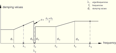
Damping is almost always specified for a mode-based procedure; see “Material damping,” Section 20.1.1. You can define a damping coefficient for all or some of the modes used in the response calculation. The damping coefficient can be given for a specified mode number or for a specified frequency range. When damping is defined by specifying a frequency range, the damping coefficient for a mode is interpolated linearly between the specified frequencies. The frequency range can be discontinuous; the average damping value will be applied for an eigenfrequency at a discontinuity. The damping coefficients are assumed to be constant outside the range of specified frequencies.
| Input File Usage: | Use the following option to define damping by specifying mode numbers: |
*MODAL DAMPING, DEFINITION=MODE NUMBERS Use the following option to define damping by specifying a frequency range: *MODAL DAMPING, DEFINITION=FREQUENCY RANGE |
| ABAQUS/CAE Usage: | Use the following input to define damping by specifying mode numbers: |
Step module: Create Step: Linear perturbation: Modal dynamics: Damping Defining damping by specifying frequency ranges is not supported in ABAQUS/CAE. |
Figure 6.3.7–1 illustrates how the damping coefficients at different eigenfrequencies are determined for the following input:
*MODAL DAMPING, DEFINITION=FREQUENCY RANGE


The following rules apply for selecting modes and specifying modal damping coefficients:
No modal damping is included by default.
Mode selection and modal damping must be specified in the same way, using either mode numbers or a frequency range.
If you do not select any modes, all modes extracted in the prior frequency analysis, including residual modes if they were activated, will be used in the superposition.
If you do not specify damping coefficients for modes that you have selected, zero damping values will be used for these modes.
Damping is applied only to the modes that are selected.
Damping coefficients for selected modes that are beyond the specified frequency range are constant and equal to the damping coefficient specified for the first or the last frequency (depending which one is closer). This is consistent with the way ABAQUS interprets amplitude definitions.
By default, the modal dynamic step will begin with zero initial displacements. If initial velocities have been defined (“Initial conditions,” Section 27.2.1), they will be used; otherwise, the initial velocities will be zero.
| Input File Usage: | *MODAL DYNAMIC, CONTINUE=NO |
| ABAQUS/CAE Usage: | Step module: Create Step: Linear perturbation: Modal dynamics: Basic: Zero initial conditions |
Alternatively, you can force the modal dynamic step to carry over the initial conditions from the immediately preceding step, which must be either another modal dynamic step or a static perturbation step:
If the immediately preceding step is a modal dynamic step, both the displacements and velocities are carried over from the end of that step and used as initial conditions for the current step.
If the immediately preceding step is a static perturbation step, the displacements are carried over from that step. If initial velocities have been defined (“Initial conditions,” Section 27.2.1), they will be used; otherwise, the initial velocities will be zero.
| Input File Usage: | *MODAL DYNAMIC, CONTINUE=YES |
| ABAQUS/CAE Usage: | Step module: Create Step: Linear perturbation: Modal dynamics: Basic: Use initial conditions |
It is not possible to prescribe nonzero displacements and rotations directly as boundary conditions (“Boundary conditions,” Section 27.3.1) in mode-based dynamic response procedures. In these procedures the motion for nodes can be specified only as base motion, as described below. Nonzero displacement or acceleration history definitions given as boundary conditions are ignored in modal superposition procedures, and any changes in the support conditions from the eigenfrequency extraction step are flagged as errors.
Boundary conditions must be applied during the eigenfrequency extraction step to the degrees of freedom that will be prescribed in the modal dynamic procedure. These degrees of freedom are grouped into one or more “bases” (see “Natural frequency extraction,” Section 6.3.5). The unnamed base is called the “primary” base. Named “secondary” bases must be defined by specifying boundary conditions in the frequency extraction step. A different motion can be prescribed for each base.
The displacements and rotations that are associated with a base are prescribed during the modal dynamic response procedure. The base motions are fully defined by at most three global translations and three global rotations. Thus, at most one base motion can be defined for each translation and rotation component. Base motions are always specified in global directions, regardless of the use of nodal transformations. You specify the global direction (1–6) for which the base motion is being defined. If a rotation is specified about an origin that is not the origin of the coordinates, you must specify the center of rotation.
The time history of a motion must be defined by an amplitude curve (“Amplitude curves,” Section 27.1.2).
| Input File Usage: | *BASE MOTION, DOF=n, AMPLITUDE=name |
| ABAQUS/CAE Usage: | Base motions are not supported in ABAQUS/CAE. |
The amplitude curve used to define the time history of the motion can be scaled. By default, the scaling factor is 1.0.
| Input File Usage: | *BASE MOTION, DOF=n, AMPLITUDE=name, SCALE=n |
| ABAQUS/CAE Usage: | Base motions are not supported in ABAQUS/CAE. |
Base motions can be defined by a displacement, a velocity, or an acceleration history. If the prescribed excitation record is given in the form of a displacement or velocity history, ABAQUS/Standard differentiates it to obtain the acceleration history. Furthermore, if the displacement or velocity histories have nonzero initial values, ABAQUS/Standard will make corrections to the initial accelerations as described in “Modal dynamic analysis,” Section 2.5.5 of the ABAQUS Theory Manual. The default is to give an acceleration history.
| Input File Usage: | Use one of the following options: |
*BASE MOTION, DOF=n, AMPLITUDE=name, TYPE=ACCELERATION *BASE MOTION, DOF=n, AMPLITUDE=name, TYPE=VELOCITY *BASE MOTION, DOF=n, AMPLITUDE=name, TYPE=DISPLACEMENT |
| ABAQUS/CAE Usage: | Base motions are not supported in ABAQUS/CAE. |
The primary base motion is specified by defining a base motion without referring to a base. If the base motion is to be applied to a secondary base, it must refer to the name of the base defined in the eigenfrequency extraction step.
| Input File Usage: | *BASE MOTION, DOF=n, AMPLITUDE=name, BASE NAME=secondary base |
| ABAQUS/CAE Usage: | Base motions are not supported in ABAQUS/CAE. |
To illustrate the concept of primary and secondary bases, consider a single-bay frame with supports at nodes 1 and 4. If the input prior to the eigenfrequency extraction step includes the following boundary conditions:
degrees of freedom 1 through 6 constrained at node 1
degree of freedom 1 constrained at node 4
degrees of freedom 3 through 6 constrained at node 4
an eigenfrequency extraction step that includes a boundary condition associated with BASE2 constraining degree of freedom 2 at node 4; and
a modal dynamic step that includes two base motion definitions: the primary base motion assigned to degree of freedom 2 that does not refer to a base and the secondary base motion assigned to degree of freedom 2 that refers to BASE2.
The degrees of freedom associated with the primary base are set to zero in the eigenfrequency extraction step, and primary base motions are introduced by multiplying the base acceleration with the modal participation factors. Hence, ABAQUS/Standard calculates the response of the structure with respect to the primary base.
The degrees of freedom associated with the secondary bases are not set to zero in the eigenfrequency extraction step; instead, a “big” mass is added to each of them. Any degree of freedom in a secondary base that was constrained by a regular boundary condition in a previous general step will be released, and a big mass will be added to that degree of freedom. Secondary base motions are introduced by nodal forces, obtained by multiplying the base acceleration with the big mass. Although the secondary base motions are defined in absolute terms, the response calculated at the secondary bases is relative to the motion of the primary base.
For a more detailed description of the base motion procedure, see “Base motions in modal-based procedures,” Section 2.5.9 of the ABAQUS Theory Manual.
The following loads can be prescribed in modal dynamic analysis, as described in “Concentrated loads,” Section 27.4.2:
Concentrated nodal forces can be applied to the displacement degrees of freedom (1–6).
Distributed pressure forces or body forces can be applied; the distributed load types available with particular elements are described in Part VI, “Elements.”
Predefined temperature fields are not allowed in transient modal dynamic analysis. Other predefined fields are ignored.
The density of the material must be defined (“Density,” Section 16.2.1). The following material properties are not active during a modal dynamic analysis: plasticity and other inelastic effects, rate-dependent material properties, thermal properties, mass diffusion properties, electrical properties (except for the electrical potential, ![]() , in piezoelectric analysis), and pore fluid flow properties. See “General and linear perturbation procedures,” Section 6.1.2.
, in piezoelectric analysis), and pore fluid flow properties. See “General and linear perturbation procedures,” Section 6.1.2.
Other than generalized axisymmetric elements with twist, any of the stress/displacement elements in ABAQUS/Standard (including those with temperature and pressure degrees of freedom) can be used in a modal dynamic analysis.
All the output variables in ABAQUS/Standard are listed in “ABAQUS/Standard output variable identifiers,” Section 4.2.1. The values of nodal solution variables U, V, and A in modal dynamics in the time domain are relative to the motion of the primary base. Hence, the sum of the relative motion and the base motion of the primary base yields the total motion; this total motion is available by requesting output variables TU, TV, and TA. In the absence of primary base motions, the relative and total motions are identical.
The following modal variables can be output to the data or results files (see “Output to the data and results files,” Section 4.1.2):
GU | Generalized displacements for all modes. |
GV | Generalized velocities for all modes. |
GA | Generalized accelerations for all modes. |
SNE | Elastic strain energy for the entire model per each mode. |
KE | Kinetic energy for the entire model per each mode. |
T | External work for the entire model per each mode. |
BM | Base motion. |
Neither element energy densities (such as the elastic strain energy density, SENER) nor whole element energies (such as the total kinetic energy of an element, ELKE) are available for output in modal dynamic analysis. However, whole model variables such as ALLIE (total strain energy) are available for mode-based procedures as output to the data or results files (see “Output to the data and results files,” Section 4.1.2).
The computational expense of a modal dynamic analysis can be decreased significantly by reducing the amount of output requested.
*HEADING
…
*AMPLITUDE, NAME=amplitude
Data lines to define amplitude variations
**
*STEP
*FREQUENCY
Data line to specify the number of modes to be extracted
*BOUNDARY
Data lines to assign degrees of freedom to the primary base
*BOUNDARY, BASE NAME=base
Data lines to assign degrees of freedom to a secondary base
*END STEP
**
*STEP
*MODAL DYNAMIC
Data line to control time incrementation
*SELECT EIGENMODES
Data lines to define the applicable mode ranges
*MODAL DAMPING
Data line to define modal damping
*BASE MOTION, DOF=dof, AMPLITUDE=amplitude
*BASE MOTION, DOF=dof, AMPLITUDE=amplitude, BASE NAME=base
*END STEP