Products: ABAQUS/Standard ABAQUS/CAE
A response spectrum analysis:
provides an estimate of the peak linear response of a structure to dynamic motion of fixed points (“base motion”);
is typically used to analyze response to a seismic event;
assumes that the system's response is linear so that it can be analyzed in the frequency domain using its natural modes, which must be extracted in a previous eigenfrequency extraction step (“Natural frequency extraction,” Section 6.3.5); and
is a linear perturbation procedure and is, therefore, not appropriate if the excitation is so severe that nonlinear effects in the system are important.
Response spectrum analysis can be used to estimate the peak response (displacement, stress, etc.) of a structure to a particular base motion. The method is only approximate, but it is often a useful, inexpensive method for preliminary design studies.
The response spectrum procedure is based on using a subset of the modes of the system, which must first be extracted by using the eigenfrequency extraction procedure. The modes will include eigenmodes and, if activated in the eigenfrequency extraction step, residual modes. The number of modes extracted must be sufficient to model the dynamic response of the system adequately, which is a matter of judgment on your part.
While the response in the response spectrum procedure is for linear vibrations, the prior response may be nonlinear. Initial stress effects (stress stiffening) will be included in the response spectrum analysis if nonlinear geometric effects (“General and linear perturbation procedures,” Section 6.1.2) were included in a general analysis step prior to the eigenfrequency extraction step.
The problem to be solved can be stated as follows: given a set of base motions, ![]() (
(![]() ), specified in orthogonal directions defined by direction cosines
), specified in orthogonal directions defined by direction cosines ![]() (
(![]() ), estimate the peak value over all time of the response of any variable in a finite element model that is simultaneously subjected to these multiple base motions. The peak response is first computed independently for each direction of excitation for each natural mode of the system as a function of frequency and damping. These independent responses are then combined to create an estimate of the actual peak response of any variable chosen for output, as a function of frequency and damping.
), estimate the peak value over all time of the response of any variable in a finite element model that is simultaneously subjected to these multiple base motions. The peak response is first computed independently for each direction of excitation for each natural mode of the system as a function of frequency and damping. These independent responses are then combined to create an estimate of the actual peak response of any variable chosen for output, as a function of frequency and damping.
The acceleration history (base motion) is not given directly in a response spectrum analysis; it must first be converted into a spectrum.
The response spectrum method is based on first finding the exact value of the peak response to each base motion of a one degree of freedom system that has a natural frequency equal to the frequency of interest. The single degree of freedom system is characterized by its undamped natural frequency, ![]() , and the fraction of critical damping present in the system,
, and the fraction of critical damping present in the system, ![]() , at each mode
, at each mode ![]() . The equations of motion of the system are integrated through time to find peak values of relative displacement, relative velocity, and absolute acceleration for the linear, one degree of freedom system. This process is repeated for all frequency and damping values in the range of interest. Plots of these responses are known as displacement, velocity, and acceleration spectra:
. The equations of motion of the system are integrated through time to find peak values of relative displacement, relative velocity, and absolute acceleration for the linear, one degree of freedom system. This process is repeated for all frequency and damping values in the range of interest. Plots of these responses are known as displacement, velocity, and acceleration spectra: ![]() ,
, ![]() , and
, and ![]() . “Analysis of a cantilever subject to earthquake motion,” Section 1.4.13 of the ABAQUS Benchmarks Manual, contains a FORTRAN program that can be used to build a spectrum from an acceleration record in this way. The response spectrum can also be obtained directly from measured data.
. “Analysis of a cantilever subject to earthquake motion,” Section 1.4.13 of the ABAQUS Benchmarks Manual, contains a FORTRAN program that can be used to build a spectrum from an acceleration record in this way. The response spectrum can also be obtained directly from measured data.
You define a response spectrum by giving a table of values of S as a function of frequency, ![]() , and damping,
, and damping, ![]() . For each damping value the magnitude of the response spectrum must be given over the entire range of frequencies needed, in ascending value of frequency. ABAQUS/Standard interpolates linearly between the values given on a log-log scale. Outside the extremes of the frequency range given, the magnitude is assumed to be constant, corresponding to the end value given. (See “Material data definition,” Section 16.1.2, for an explanation of data interpolation.)
. For each damping value the magnitude of the response spectrum must be given over the entire range of frequencies needed, in ascending value of frequency. ABAQUS/Standard interpolates linearly between the values given on a log-log scale. Outside the extremes of the frequency range given, the magnitude is assumed to be constant, corresponding to the end value given. (See “Material data definition,” Section 16.1.2, for an explanation of data interpolation.)
Any number of spectra can be defined, and each spectrum must be named. The response spectrum procedure allows up to three spectra to be applied to the model in orthogonal physical directions defined by their direction cosines.
| Input File Usage: | *SPECTRUM, NAME=name |
Repeat this option to define multiple spectra for an analysis. |
| ABAQUS/CAE Usage: | To define a spectrum in ABAQUS/CAE, you must use the Keywords Editor to add the *SPECTRUM option to your input file. To apply a spectrum to the model, do the following: |
Step module: Create Step: Linear perturbation: Response spectrum: Use response spectrum: enter the spectrum name in the text field next to the physical direction in which it should be applied |
You must indicate whether a displacement, velocity, or acceleration spectrum is given. The default is a displacement spectrum. An acceleration spectrum can be given in g-units. In this case you must also specify the value of the acceleration of gravity.
| ABAQUS/CAE Usage: | In ABAQUS/CAE you must use the Keywords Editor to add the *SPECTRUM option to your input file. |
The data for the spectrum can be specified in an alternate input file and read into the ABAQUS/Standard input file.
| Input File Usage: | *SPECTRUM, NAME=name, INPUT=file name |
| ABAQUS/CAE Usage: | In ABAQUS/CAE you must use the Keywords Editor to add the *SPECTRUM option to your input file. |
Since the response spectrum procedure uses modal methods to define a model's response, the value of any physical variable is defined from the amplitudes of the modal responses (the “generalized coordinates”), ![]() . The first stage in the response spectrum procedure is to estimate the peak values of these modal responses. For mode
. The first stage in the response spectrum procedure is to estimate the peak values of these modal responses. For mode ![]() and spectrum k this is
and spectrum k this is
![]()
![]()
is the modal amplitude for mode ![]() ;
;
![]()
is a scaling parameter introduced as part of the response spectrum procedure definition for spectrum ![]() ;
;
![]()
is the user-defined value of the spectrum (see “Defining a spectrum”) in direction k interpolated, if necessary, at natural frequency ![]() and the fraction of critical damping
and the fraction of critical damping ![]() in mode
in mode ![]() ;
;
![]()
is the jth direction cosine for the kth spectrum; and
![]()
is the participation factor for mode ![]() in direction j (see “Natural frequency extraction,” Section 6.3.5).
in direction j (see “Natural frequency extraction,” Section 6.3.5).
Similar expressions for ![]() and
and ![]() can be obtained by substituting velocity or acceleration spectra in the above equation.
can be obtained by substituting velocity or acceleration spectra in the above equation.
The individual peak responses to the excitations in different directions will occur at different times and, therefore, must be combined into an overall peak response. Two combinations must be performed, and both introduce approximations into the results:
The multidirectional excitations must be combined into one overall response. This combination is controlled by the directional summation method, as described below in “Directional summation methods.”
The peak modal responses must be combined to estimate the peak physical response. This combination is controlled by the modal summation method, as described below in “Modal summation methods.”
You choose the method for combining the multidirectional excitations depending on the nature of the excitations.
If the input spectra in the different directions are components of a base excitation that is approximately in a single direction in space, then for each mode the peak responses in the different spatial directions are summed algebraically by
![]()
| Input File Usage: | Use the following option to choose the algebraic summation approach: |
*RESPONSE SPECTRUM, COMP=ALGEBRAIC, SUM=sum |
| ABAQUS/CAE Usage: | Step module: Create Step: Linear perturbation: Response spectrum: Excitations: Single direction |
If the spectra in different directions represent independent excitations, the modal summation is performed first, as explained below in “Modal summation methods.” Then the responses in different excitation directions are combined by
| Input File Usage: | Use the following option to choose the square root of the sum of the squares summation approach: |
*RESPONSE SPECTRUM, COMP=SRSS, SUM=sum |
| ABAQUS/CAE Usage: | Step module: Create Step: Linear perturbation: Response spectrum: Excitations: Multiple direction square root of the sum of squares |
The peak response of some physical variable ![]() (a component i of displacement, stress, section force, reaction force, etc.) caused by the motion in the
(a component i of displacement, stress, section force, reaction force, etc.) caused by the motion in the ![]() th natural mode excited by the given response spectra in direction k at frequency
th natural mode excited by the given response spectra in direction k at frequency ![]() with damping
with damping ![]() is given by
is given by
![]()
There are several methods for combining these peak physical responses in the individual modes, ![]() , into estimates of the total peak response,
, into estimates of the total peak response, ![]() . Some of the methods implemented in ABAQUS/Standard were recommended by the Regulatory Guide 1.92 of the U.S. Nuclear Regulatory Commission issued in 1976. The updated documents, “Reevaluation of Regulatory Guidance on Modal Response Combination Methods for Seismic Response Spectrum Analysis,” was issued in 1999 (NUREG/CR-6645, BNL-NUREG-52276) and “Draft Regulatory Guide” (DG-1127) issued in 2005 contain new recommendations. You are advised to read the new recommendations before choosing a modal summation method from among those described below.
. Some of the methods implemented in ABAQUS/Standard were recommended by the Regulatory Guide 1.92 of the U.S. Nuclear Regulatory Commission issued in 1976. The updated documents, “Reevaluation of Regulatory Guidance on Modal Response Combination Methods for Seismic Response Spectrum Analysis,” was issued in 1999 (NUREG/CR-6645, BNL-NUREG-52276) and “Draft Regulatory Guide” (DG-1127) issued in 2005 contain new recommendations. You are advised to read the new recommendations before choosing a modal summation method from among those described below.
The absolute value method is the most conservative method for combining the modal responses. It is obtained by summing the absolute values resulting from each mode:
![]()
| Input File Usage: | *RESPONSE SPECTRUM, COMP=comp, SUM=ABS |
| ABAQUS/CAE Usage: | Step module: Create Step: Linear perturbation: Response spectrum: Summations: Absolute values |
The square root of the sum of the squares method is less conservative than the absolute value method. It is also usually more accurate if the natural frequencies of the system are well separated. It uses the square root of the sum of the squares to combine the modal responses:
| Input File Usage: | *RESPONSE SPECTRUM, COMP=comp, SUM=SRSS |
| ABAQUS/CAE Usage: | Step module: Create Step: Linear perturbation: Response spectrum: Summations: Square root of the sum of squares |
The absolute value and square root of the sum of the squares methods can be combined to yield the Naval Research Laboratory method. It distinguishes the mode, ![]() , in which the physical variable has its maximum response and adds the square root of the sum of squares of the peak responses in all other modes to the absolute value of the peak response of that mode. This method gives the estimate:
, in which the physical variable has its maximum response and adds the square root of the sum of squares of the peak responses in all other modes to the absolute value of the peak response of that mode. This method gives the estimate:
| Input File Usage: | *RESPONSE SPECTRUM, COMP=comp, SUM=NRL |
| ABAQUS/CAE Usage: | Step module: Create Step: Linear perturbation: Response spectrum: Summations: Naval Research Laboratory |
The ten-percent method recommended by Regulatory Guide 1.92 (1976) is no longer recommended according to the “Reevaluation of Regulatory Guidance on Modal Response Combination Methods for Seismic Response Spectrum Analysis” document issued in 1999. It is retained here because of its extensive prior use. The ten-percent method modifies the square root of the sum of the squares method by adding a contribution from all pairs of modes ![]() and
and ![]() whose frequencies are within 10% of each other, giving the estimate:
whose frequencies are within 10% of each other, giving the estimate:
![]()
The ten-percent method reduces to the square root of the sum of the squares method if the modes are well separated with no coupling between them.
| Input File Usage: | *RESPONSE SPECTRUM, COMP=comp, SUM=TENP |
| ABAQUS/CAE Usage: | Step module: Create Step: Linear perturbation: Response spectrum: Summations: Ten percent |
Like the ten-percent method, the complete quadratic combination method improves the estimation for structures with closely spaced eigenvalues. The complete quadratic combination method combines the modal response with the formula
If the modes are well spaced, their cross-correlation coefficient will be small (![]() ) and the method will give the same results as the square root of the sum of the squares method.
) and the method will give the same results as the square root of the sum of the squares method.
This method is usually recommended for asymmetrical building systems since, in such cases, other methods can underestimate the response in the direction of motion and overestimate the response in the transverse direction.
| Input File Usage: | *RESPONSE SPECTRUM, COMP=comp, SUM=CQC |
| ABAQUS/CAE Usage: | Step module: Create Step: Linear perturbation: Response spectrum: Summations: Complete quadratic combination |
You can select the modes to be used in modal superposition and specify damping values for all selected modes.
You can select modes by specifying the mode numbers individually, by requesting that ABAQUS/Standard generate the mode numbers automatically, or by requesting the modes that belong to specified frequency ranges. If you do not select the modes, all modes extracted in the prior eigenfrequency extraction step, including residual modes if they were activated, are used in the modal superposition.
| Input File Usage: | Use one of the following options to select the modes by specifying mode numbers: |
*SELECT EIGENMODES, DEFINITION=MODE NUMBERS
*SELECT EIGENMODES, GENERATE, DEFINITION=MODE NUMBERS
Use the following option to select the modes by specifying a frequency range: *SELECT EIGENMODES, DEFINITION=FREQUENCY RANGE |
| ABAQUS/CAE Usage: | You cannot select the modes in ABAQUS/CAE; all modes extracted are used in the modal superposition. |
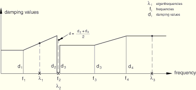
Damping is almost always specified for a mode-based procedure; see “Material damping,” Section 20.1.1. You can define a damping coefficient for all or some of the modes used in the response calculation. The damping coefficient can be given for a specified mode number or for a specified frequency range. When damping is defined by specifying a frequency range, the damping coefficient for an mode is interpolated linearly between the specified frequencies. The frequency range can be discontinuous; the average damping value will be applied for an eigenfrequency at a discontinuity. The damping coefficients are assumed to be constant outside the range of specified frequencies.
| Input File Usage: | Use the following option to define damping by specifying mode numbers: |
*MODAL DAMPING, DEFINITION=MODE NUMBERS Use the following option to define damping by specifying a frequency range: *MODAL DAMPING, DEFINITION=FREQUENCY RANGE |
| ABAQUS/CAE Usage: | Use the following input to define damping by specifying mode numbers: |
Step module: Create Step: Linear perturbation: Response spectrum: Damping Defining damping by specifying frequency ranges is not supported in ABAQUS/CAE. |
Figure 6.3.10–1 illustrates how the damping coefficients at different eigenfrequencies are determined for the following input:
*MODAL DAMPING, DEFINITION=FREQUENCY RANGE


The following rules apply for selecting modes and specifying modal damping coefficients:
No modal damping is included by default.
Mode selection and modal damping must be specified in the same way, using either mode numbers or a frequency range.
If you do not select any modes, all modes extracted in the prior frequency analysis, including residual modes if they were activated, will be used in the superposition.
If you do not specify damping coefficients for modes that you have selected, zero damping values will be used for these modes.
Damping is applied only to the modes that are selected.
Damping coefficients for selected modes that are beyond the specified frequency range are constant and equal to the damping coefficient specified for the first or the last frequency (depending which one is closer). This is consistent with the way ABAQUS interprets amplitude definitions.
It is not appropriate to specify initial conditions in a response spectrum analysis.
All points constrained by boundary conditions and the ground nodes of connector elements are assumed to move in phase in any one direction. This base motion can use a different input spectrum in each of three orthogonal directions (two directions in a two-dimensional model). You define the input spectra, ![]() , as functions of frequency,
, as functions of frequency, ![]() , for different values of critical damping,
, for different values of critical damping, ![]() , as described earlier in “Defining a spectrum.” Secondary bases cannot be used in a response spectrum analysis.
, as described earlier in “Defining a spectrum.” Secondary bases cannot be used in a response spectrum analysis.
The only “loading” that can be defined in a response spectrum analysis is that defined by the input spectra, as described earlier. No other loads can be prescribed in a response spectrum analysis.
Predefined fields, including temperature, cannot be used in response spectrum analysis.
The density of the material must be defined (“Density,” Section 16.2.1). The following material properties are not active during a response spectrum analysis: plasticity and other inelastic effects, rate-dependent material properties, thermal properties, mass diffusion properties, electrical properties, and pore fluid flow properties—see “General and linear perturbation procedures,” Section 6.1.2.
Other than generalized axisymmetric elements with twist, any of the stress/displacement elements in ABAQUS/Standard can be used in a response spectrum analysis—see “Choosing the appropriate element for an analysis type,” Section 21.1.3.
All the output variables in ABAQUS/Standard are listed in “ABAQUS/Standard output variable identifiers,” Section 4.2.1. The value of an output variable such as strain, E; stress, S; or displacement, U, is its peak magnitude.
In addition to the usual output variables available, the following modal variables are available for response spectrum analysis and can be output to the data and/or results files (see “Output to the data and results files,” Section 4.1.2):
GU | Generalized displacements for all modes. |
GV | Generalized velocities for all modes. |
GA | Generalized accelerations for all modes. |
SNE | Elastic strain energy for the entire model per each mode. |
KE | Kinetic energy for the entire model per each mode. |
T | External work for the entire model per each mode. |
Neither element energy densities (such as the elastic strain energy density, SENER) nor whole element energies (such as the total kinetic energy of an element, ELKE) are available for output in response spectrum analysis. However, whole model variables such as ALLIE (total strain energy) are available for modal-based procedures as output to the data and/or results files (see “Output to the data and results files,” Section 4.1.2).
*HEADING … *BOUNDARY Data lines to define points to be excited by the base motion controlled by the input spectra *SPECTRUM, NAME=name1, TYPE=type Data lines to define spectrum “name1” as a function of frequency,, and fraction of critical damping,
*SPECTRUM, NAME=name2, TYPE=type Data lines to define spectrum “name2” as a function of frequency,