Products: ABAQUS/Standard ABAQUS/Explicit
A distribution:
is a spatially varying field (of scalars, shell stiffness matrices, or orientations) defined over elements or nodes in an ABAQUS model;
can be referred to by name to define element properties on an element-by-element basis as described in “Assigning element properties on an element-by-element basis,” Section 21.1.5; and
can be referred to by name to specify initial contact clearances as described in “Resolving initial overclosures and specifying initial clearances for general contact,” Section 29.3.5.
A distribution is a spatial analogy of an amplitude definition (see “Amplitude curves,” Section 27.1.2). Whereas amplitude definitions can be referred to by name to provide arbitrary time variations of loads, displacements, and other prescribed variables, distributions can be referred to by name to specify arbitrary spatial variations of selected element properties (see “Assigning element properties on an element-by-element basis,” Section 21.1.5) or spatial variations of initial contact clearances (see “Resolving initial overclosures and specifying initial clearances for general contact,” Section 29.3.5).
The two main components of a distribution are its location and field data. The location identifies where the distribution is defined, either on elements or nodes. Field data are data of a specific algebraic type (such as a scalar). A distribution is defined by specifying field data (of the same type but not necessarily the same value) for each node or element included in the distribution definition.
To define a distribution, you must assign it a unique name. You must specify where the distribution is defined; i.e., its location. You must also specify the algebraic type of the data to be distributed onto the specified elements or nodes.
| Input File Usage: | *DISTRIBUTION, NAME=name, LOCATION=distribution location label, TYPE=field type label element or node set or number, field data |
There is no limit on the number of distributions to which a given element or node may belong. If an element or node is specified more than once in a given distribution definition, the last specification given is used. Elements and nodes cannot be combined within the same distribution definition.
Defining a distribution on elements requires you to specify field data for each element or element set included in the distribution definition.
| Input File Usage: | *DISTRIBUTION, LOCATION=ELEMENT element set or element number, field data |
Defining a distribution on nodes requires you to specify field data for each node or node set included in the distribution definition.
| Input File Usage: | *DISTRIBUTION, LOCATION=NODE node set or node number, field data |
Three types of algebraic data are available to define scalar, shell stiffness matrix, and orientation distributions. Field data of different algebraic types cannot be included in the same distribution definition.
A scalar distribution requires you to specify a floating point scalar for each element or node included in the distribution definition.
| Input File Usage: | *DISTRIBUTION, TYPE=SCALAR element or node set or number, scalar data |
A shell stiffness distribution requires you to specify 21 floating point components of a symmetric positive definite shell stiffness matrix for each shell element included in the distribution definition. Shell stiffness distributions defined on non-shell elements will be ignored.
The matrix components for a symmetric shell stiffness matrix ![]() should be given in the order
should be given in the order ![]() ,
, ![]() ,
, ![]() ,
, ![]() ,
, ![]() ,
, ![]() ,
, ![]() ,...,
,..., ![]() ,
, ![]() ,...,
,..., ![]() ,...,
,..., ![]() ,...,
,..., ![]() .
.
| Input File Usage: | *DISTRIBUTION, TYPE=SHELL3D STIFFNESS element set or element number, 21 matrix components |
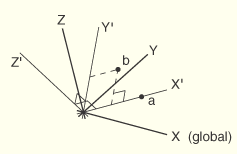
An orientation distribution requires you to specify the coordinates of two points that define a rectangular Cartesian coordinate system for each element included in the distribution definition. Orientation distributions can be defined only on elements.
A rectangular coordinate system is defined by its origin and the two points, a and b, shown in Figure 2.7.1–1. Point a must be on the local ![]() -axis, and point b must be in the
-axis, and point b must be in the ![]() -
-![]() plane. Although it is not necessary, it is intuitive to select point b such that it is on or near the local
plane. Although it is not necessary, it is intuitive to select point b such that it is on or near the local ![]() -axis.
-axis.
| Input File Usage: | *DISTRIBUTION, NAME=name, TYPE=ORIENTATION element set or element number, |
In the following simple example three different distributions (DIST1, DIST2, and DIST3) are defined. DIST1 is a scalar distribution that is associated with element set ESET1, which contains elements 1 through 4. The scalar values assigned to elements 1, 2, 3, and 4 are 2.0, 1.0, 4.0, and 3.0, respectively. Element 1 is included twice in the data lines for DIST1, first in the element set ESET2, and then as an individual element. The last specified value (2.0) is used for element 1. DIST2 is a distribution of orientations that is associated with element set ESET2, which contains elements 1 and 2. A local coordinate system that coincides with the global ![]() coordinate system is defined for element 1. A local coordinate system whose local X-, Y-, and Z-directions coincide with the global Y-, Z-, and X- directions, respectively, is defined for element 2. DIST3 is a scalar distribution that is associated with node set NSET1, which contains nodes 10, 20, and 40. The scalar values assigned to nodes 10, 20, and 40 are 100.0, 200.0, and 400.0, respectively.
coordinate system is defined for element 1. A local coordinate system whose local X-, Y-, and Z-directions coincide with the global Y-, Z-, and X- directions, respectively, is defined for element 2. DIST3 is a scalar distribution that is associated with node set NSET1, which contains nodes 10, 20, and 40. The scalar values assigned to nodes 10, 20, and 40 are 100.0, 200.0, and 400.0, respectively.
*ELSET, ELSET=ESET1
 1, 4
*ELSET, ELSET=ESET2
 1, 2
*NSET, NSET=NSET1
 10, 20, 40
*DISTRIBUTION, NAME=DIST1, LOCATION=ELEMENT, TYPE=SCALAR
 ESET2, 1.
 1, 2.
 3, 4.
 4, 3.
*DISTRIBUTION, NAME=DIST2, LOCATION=ELEMENT,  TYPE=ORIENTATION
 1, 1., 0., 0., 0., 1., 0.
 2, 0., 1., 0., 0., 0., 1.
*DISTRIBUTION, NAME=DIST3, LOCATION=NODE, TYPE=SCALAR
 10, 100.
 20, 200.
 40, 400.