In this example you will solve the channel forming problem from Chapter 12, “Contact,” using ABAQUS/Explicit. You will then compare the results from the ABAQUS/Standard and ABAQUS/Explicit analyses.
You will make modifications to the model created for the ABAQUS/Standard analysis so that you are able to run it in ABAQUS/Explicit. These modifications include adding density to the material model, changing the element library, and changing the steps. Before running the ABAQUS/Explicit analysis, you will use the frequency extraction procedure in ABAQUS/Standard to determine the time period required to obtain a proper quasi-static response.
Use ABAQUS/CAE to modify the model for this simulation. A Python script is provided in “Forming a channel,” Section A.12. When this script is run through ABAQUS/CAE, it creates the complete analysis model for this problem. Run this script if you encounter difficulties following the instructions given below or if you wish to check your work. Instructions on how to fetch and run the script are given in Appendix A, “Example Files.”
Before starting, open the model database file for the channel forming example created in “ABAQUS/Standard example: forming a channel,” Section 12.6.
Determining an appropriate step time
“Loading rates,” Section 13.2, discusses the procedures for determining the appropriate step time for a quasi-static process. We can determine an approximate lower bound on step time duration if we know the lowest natural frequency, the fundamental frequency, of the blank. One way to obtain such information is to run a frequency analysis in ABAQUS/Standard. In this forming analysis the punch deforms the blank into a shape similar to the lowest mode. Therefore, it is important that the time for the first forming stage is greater than or equal to the time period for the lowest mode if you wish to model structural, as opposed to localized, deformation.
To perform a natural frequency extraction:
Copy the existing model to a model named Frequency. Make all of the following changes to the Frequency model. In the frequency extraction analysis you will replace all existing steps with a single frequency extraction step. In addition, you will delete all of the rigid body tools and contact interactions; they are not necessary for determining the fundamental frequency of the blank.
Add a density of 7800 to the material model Steel.
Delete the die, holder, and punch part instances. These rigid parts are not necessary for the frequency analysis.
Tip: You can delete any part instance using the Model Tree by expanding Instances underneath the Assembly container, clicking mouse button 3 on the instance name, and selecting Delete from the menu that appears.
Replace the existing steps with a single frequency extraction step.
Delete the steps Remove Right Constraint, Holder Force, Establish Contact II, and Move Punch.
In the Model Tree, click mouse button 3 on the step Establish Contact I and select Replace from the menu that appears.
In the Replace Step dialog box, select Frequency from the list of available Linear perturbation procedures. Enter the step description Frequency modes; select the Lanczos eigensolver option; and request five eigenvalues. Rename the step Extract Frequencies.
Suppress the DOF Monitor.
Note: Since the frequency extraction step is a linear perturbation procedure, nonlinear material properties will be ignored. In this analysis the left end of the blank is constrained in the x-direction and cannot rotate about the normal; however, it is not constrained in the y-direction. Therefore, the first mode extracted will be a rigid body mode. The frequency of the second mode will determine the appropriate time period for the quasi-static analysis in ABAQUS/Explicit.
Delete all contact interactions.
Open the Boundary Condition Manager, and examine the boundary conditions in the Extract Frequencies step. Delete all boundary conditions except the boundary condition named CenterBC. This leaves the blank constrained with a symmetry boundary condition applied to the left end.
Remesh the blank if necessary.
Create a job named Forming-Frequency with the following job description: Channel forming -- frequency analysis. Submit the job for analysis, and monitor the solution progress.
When the analysis is complete, enter the Visualization module and open the output database file created by this job. From the main menu bar, select Plot![]() Deformed Shape; or use the
Deformed Shape; or use the ![]() tool in the toolbox.
tool in the toolbox.
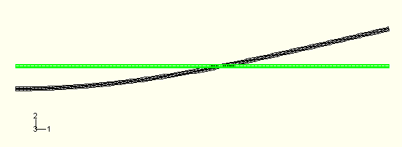
The deformed model shape for the first buckling mode is plotted. Advance the plot to the second mode of the blank. Superimpose the undeformed model shape on the deformed model shape.
The frequency analysis shows that the blank has a fundamental frequency of 140 Hz, corresponding to a period of 0.00714 s. Figure 13–8 shows the displaced shape of the second mode. We now know that the shortest step time for the forming analysis is 0.00714 s.
Creating the ABAQUS/Explicit forming analysis
The goal of the forming process is to quasi-statically form a channel with a punch displacement of 0.03 m. In selecting loading rates for quasi-static analyses, it is recommended that you begin with faster loading rates and decrease the loading rates as necessary to converge on a quasi-static solution more quickly. However, if you wish to increase the likelihood of a quasi-static result in your first analysis attempt, you should consider step times that are a factor of 10 to 50 times slower than that corresponding to the fundamental frequency. In this analysis you will start with a time period of 0.007 s for the forming analysis step. This is based on the frequency analysis performed in ABAQUS/Standard, which shows that the blank has a fundamental frequency of 140 Hz, corresponding to a time period of 0.00714 s. This time period corresponds to a constant punch velocity of 4.3 m/s. You will examine the kinetic and internal energy results carefully to check that the solution does not include significant dynamic effects.
Copy the Standard model to a model named Explicit. Make all subsequent model changes to the Explicit model. To begin, edit the Steel material definition to include a mass density of 7800 kg/m3.
In the ABAQUS/Standard analysis an initial gap is modeled between the punch and the blank to aid the contact calculations. It is not necessary to take this precaution in the ABAQUS/Explicit analysis. Therefore, in the Assembly module, translate the punch –0.001 m in the U2 direction. Click Yes in the warning dialog box that appears regarding relative and absolute constraints.
A concentrated force is applied to the blank holder. To compute the dynamic response of the holder, a point mass must be assigned to its rigid body reference point. The actual mass of the holder is not important; what is important is that the mass should be of the same order of magnitude as the mass of the blank (0.78 kg) to minimize noise in the contact calculations. Choose a point mass value of 0.1 kg. To assign the mass, expand Engineering Features underneath the Assembly container in the Model Tree. In the list that appears, double-click Inertias. In the Create Inertia dialog box that appears, enter the name PointMass and click Continue. Select the set RefHolder, and assign it a mass of 0.1 kg.
You need to create two steps for the ABAQUS/Explicit analysis. In the first step the holder force is applied; in the second step the punch stroke is applied. Delete all steps except the step named Establish Contact I. Replace this step with a single explicit dynamics step. Enter the step description Apply holder force, and specify a time period of 0.0001 s. This time period is appropriate for the application of the holder force because it is long enough to avoid dynamic effects but short enough to prevent a significant impact on the run time for the job. Rename this step Holder force. Create a second explicit dynamics step named Displace punch with a time period of 0.007 s. Enter Apply punch stroke as the step description.
To help determine how closely the analysis approximates the quasi-static assumption, the various energy histories will be useful. Especially useful is comparing the kinetic energy to the internal strain energy. The energy history is written to the output database file by default.
For the first attempt of this metal forming analysis, you will use tabular amplitude curves with the default smoothing parameter for both the application of the holder force and the punch stroke. Create a tabular amplitude curve for application of the holder force named Ramp1. Enter the amplitude data in Table 13–1. Define a second tabular amplitude curve for the punch stroke named Ramp2. Enter the amplitude data in Table 13–2.
Open the Load Manager, and create a concentrated force named RefHolderForce in the step named Holder force. Specify RefHolder for the point of application and a magnitude of -440000 in the CF2 direction. Change the amplitude definition for this load to Ramp1.
Open the Boundary Condition Manager, and delete the boundary conditions named MidLeftBC and MidRightBC. Edit the RefDieBC boundary condition so that the constraint in the U2 direction is zero in the Holder force step. Do not change the constraints in the other directions. Remove the constraint in the U2 direction for the RefHolderBC boundary condition, and leave the constraints in the other directions unchanged. Change the displacement boundary condition RefPunchBC in the U2 direction to –0.03 m in the Displace Punch step. Use the amplitude curve Ramp2 for this boundary condition.
Monitoring the value of a degree of freedom
In this model you will monitor the vertical displacement (degree of freedom 2) of the punch's reference node throughout the step. Because the DOF Monitor was set to monitor the vertical displacement of RefPunch in the ABAQUS/Standard forming analysis, you do not need to make any changes.
Mesh creation and job definition
Change the family of the elements used to mesh the blank to Explicit, and specify enhanced hourglass control. Mesh the blank. The tools have been modeled with analytical surfaces so they do not need to be meshed.
Create a job named Forming-1. Give the job the following description: Channel forming -- attempt 1.
Before you run the forming analysis, you may wish to know how many increments the analysis will take and, consequently, how much computer time the analysis requires. You can run a data check analysis to obtain the approximate value for the initial stable time increment, or you can estimate it using the relations in “Mass scaling,” Section 13.3. Knowing the stable time increment, which in this case does not change much from increment to increment, you can determine how many increments are required to complete the forming stage. Once the analysis begins, you can get an idea of how much CPU time is required per increment and, consequently, how much CPU time the analysis requires.
Using the relations stated in “Mass scaling,” Section 13.3, the stable time increment for this analysis is approximately 1 × 10⁻⁷ s. Therefore, the forming stage requires approximately 185,000 increments for a step time of 0.007 s.
Save your model to a model database file, and submit the job for analysis. Monitor the solution progress; correct any modeling errors that are detected, and investigate the cause of any warning messages. Ten minutes or more may be required to run this analysis to completion.
Once the analysis is underway, an X–Y plot of the values of the degree of freedom that you selected to monitor (the punch's vertical displacement) appears in a separate viewport. From the main menu bar, select Viewport![]() Job Monitor: Forming-1 to follow the progression of the punch's displacement in the 2-direction over time as the analysis runs.
Job Monitor: Forming-1 to follow the progression of the punch's displacement in the 2-direction over time as the analysis runs.
Strategy for evaluating the results
Before looking at the results that are ultimately of interest, such as stresses and deformed shapes, we need to determine whether or not the solution is quasi-static. One good approach is to compare the kinetic energy history to the internal energy history. In a metal forming analysis most of the internal energy is due to plastic deformation. In this model the blank is the primary source of kinetic energy (the motion of the holder is negligible, and the punch and die have no mass associated with them). To determine whether an acceptable quasi-static solution has been obtained, the kinetic energy of the blank should be no greater than a few percent of its internal energy. For greater accuracy, especially when springback stresses are of interest, the kinetic energy should be lower. This approach is very useful because it applies to all types of metal forming processes and does not require any intuitive understanding of the stresses in the model; many forming processes may be too complex to permit an intuitive feel for the results.
While a good primary indication of the caliber of a quasi-static analysis, the ratio of kinetic energy to internal energy alone is not adequate to confirm the quality. You should also evaluate the two energies independently to determine whether they are reasonable. This part of the evaluation takes on increased importance when accurate springback stress results are needed because an accurate springback stress solution is highly dependent on accurate plasticity results. Even if the kinetic energy is fairly small, if it contains large oscillations, the model could be experiencing significant plasticity. Generally, we expect smooth loading to produce smooth results; if the loading is smooth but the energy results are oscillatory, the results may be inadequate. Since an energy ratio is incapable of showing such behavior, you should also study the kinetic energy history itself to see whether it is smooth or noisy.
If the kinetic energy does not indicate quasi-static behavior, it can be useful to look at velocity histories at some nodes to get an understanding of the model's behavior in various regions. Such velocity histories can indicate which regions of the model are oscillating and causing the high kinetic energies.
Evaluating the results
Enter the Visualization module, and open the output database created by this job (Forming-1.odb). Plot the whole model kinetic (ALLKE) and internal (ALLIE) energies.
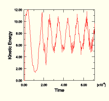
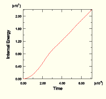
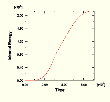
History plots of the kinetic and internal energies for the whole model appear as shown in Figure 13–9 and Figure 13–10, respectively.
The kinetic energy history shown in Figure 13–9 oscillates significantly. In addition, the kinetic energy history has no clear relation to the forming of the blank, which indicates the inadequacy of this analysis. In this analysis the punch velocity remains constant, while the kinetic energy—which is primarily due to the motion of the blank—is far from constant.
Comparing Figure 13–9 and Figure 13–10 shows that the kinetic energy is a small fraction (less than 1%) of the internal energy through all but the very beginning of the analysis. The criterion that kinetic energy must be small relative to internal energy has been satisfied, even for this severe loading case.
Although the kinetic energy of the model is a small fraction of the internal energy, it is still quite noisy. Therefore, we should change the simulation in some way to obtain a smoother response.
Even if the punch actually moves at a nearly constant velocity, the results of the first simulation attempt indicate it is desirable to use a different amplitude curve that allows the blank to accelerate more smoothly. When considering what type of loading amplitude to use, remember that smoothness is important in all aspects of a quasi-static analysis. The preferred approach is to move the punch as smoothly as possible the desired distance in the desired amount of time.
We will now analyze the forming stage using a smoothly applied punch force and a smoothly applied punch displacement; we will compare the results to those obtained earlier. Refer to “Smooth amplitude curves,” Section 13.2.1, for an explanation of the smooth step amplitude curve.
Define a smooth step amplitude curve named Smooth1. Enter the amplitude data given in Table 13–1. Create a second smooth step amplitude curve named Smooth2 using the amplitude data given in Table 13–2. Modify the RefHolderForce load in the Holder force step so that it refers to the Smooth1 amplitude. Modify the displacement boundary condition RefPunchBC in the Displace punch step so that it refers to the Smooth2 amplitude. By specifying an amplitude of 0.0 at the beginning of the step and an amplitude of 1.0 at the end of the step, ABAQUS/Explicit creates an amplitude definition that is smooth in both its first and second derivatives. Therefore, using a smooth step amplitude curve for the displacement control also assures us that the velocity and acceleration are smooth.
Create a job named Forming-2. Give the job the following description: Channel forming -- attempt 2.
Save your model, and submit the job for analysis. Monitor the solution progress; correct any modeling errors that are detected, and investigate the cause of any warning messages. Ten minutes or more may be required to run this analysis to completion.
Evaluating the results for attempt 2
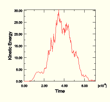
The kinetic energy history is shown in Figure 13–11. The response of the kinetic energy is clearly related to the forming of the blank: the value of kinetic energy peaks in the middle of the second step, corresponding to the time when the punch velocity is the greatest. Thus, the kinetic energy is appropriate and reasonable.
The internal energy for attempt 2, shown in Figure 13–12, shows a smooth increase from zero up to the final value. Again, the ratio of kinetic energy to internal energy is quite small and appears to be acceptable.
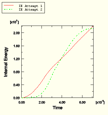
Figure 13–13 compares the internal energy in the two forming attempts.Our initial criteria for evaluating the acceptability of the results was that the kinetic energy should be small compared to the internal energy. What we found was that even for the most severe case, attempt 1, this condition seems to have been met adequately. The addition of a smooth step amplitude curve helped reduce the oscillations in the kinetic energy, yielding a satisfactory quasi-static response.
The additional requirements—that the histories of kinetic energy and internal energy must be appropriate and reasonable—are very useful and necessary, but they also increase the subjectivity of evaluating the results. Enforcing these requirements in general for more complex forming processes may be difficult because these requirements demand some intuition regarding the behavior of the forming process.
Results of the forming analysis
Now that we are satisfied that the quasi-static solution for the forming analysis is adequate, we can study some of the other results of interest. Figure 13–14 shows a comparison of the Mises stress in the blank obtained with ABAQUS/Standard and ABAQUS/Explicit.
Figure 13–14 Contour plot of Mises stress in ABAQUS/Standard (left) and ABAQUS/Explicit (right) channel forming analyses.
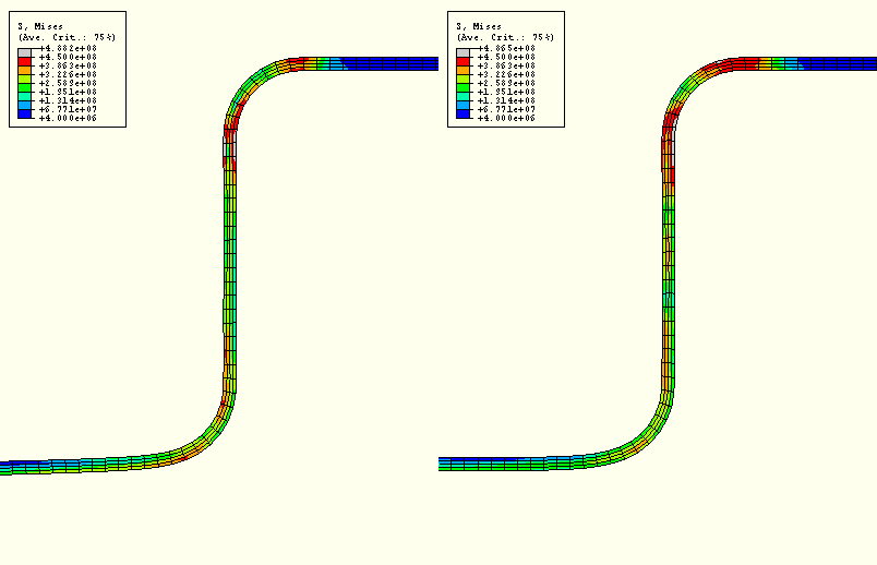
The plot shows that the peak stresses in the ABAQUS/Standard and ABAQUS/Explicit analyses are within 1% of each other and that the overall stress contours of the blank are very similar. To further examine the validity of the quasi-static analysis results, you should compare the equivalent plastic strain results and final deformed shapes from the two analyses.
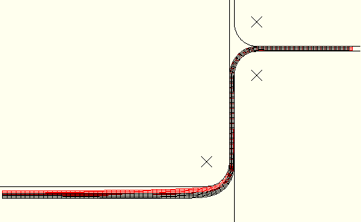
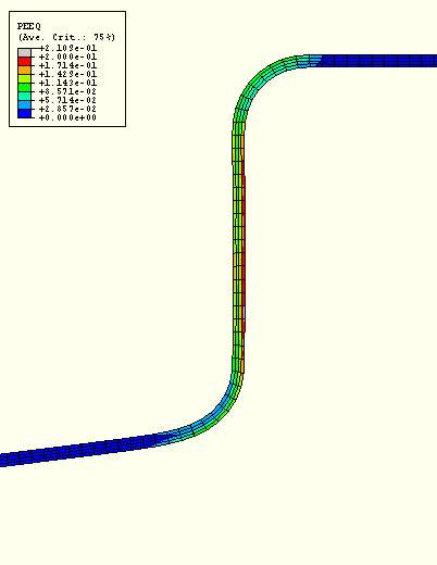
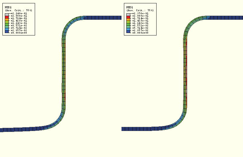
Figure 13–15 shows contour plots of the equivalent plastic strain in the blank, and Figure 13–16 shows an overlay plot of the final deformed shape predicted by the two analyses.
Figure 13–15 Contour plot of PEEQ in ABAQUS/Standard (left) and ABAQUS/Explicit (right) channel forming analyses.
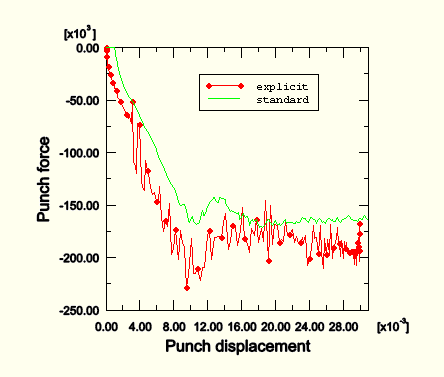
You should also compare the steady punch force predicted by the ABAQUS/Standard and ABAQUS/Explicit analyses. As seen in Figure 13–17, the steady punch force predicted by ABAQUS/Explicit is approximately 12% higher than that predicted by ABAQUS/Standard. The differences between the ABAQUS/Standard and ABAQUS/Explicit results are primarily due to two factors. First, ABAQUS/Explicit regularizes the material data. Second, friction effects are handled slightly differently in the two analysis products; ABAQUS/Standard uses penalty friction, whereas ABAQUS/Explicit uses kinematic friction.
From these comparisons it is clear that both ABAQUS/Standard and ABAQUS/Explicit are capable of handling difficult contact analyses such as this one. However, there are some advantages to running this type of analysis in ABAQUS/Explicit: ABAQUS/Explicit is able to handle complex contact conditions more readily and with fewer manipulations of steps and boundary conditions than ABAQUS/Standard. In particular, the ABAQUS/Standard analysis requires five steps and additional boundary conditions to ensure the proper contact conditions and prevent rigid body motions. In ABAQUS/Explicit the same analysis is completed using only two steps and no extra boundary conditions. However, when choosing ABAQUS/Explicit for quasi-static analysis, you should be aware that you may need to iterate on an appropriate loading rate. In determining the loading rate, it is recommended that you begin with faster loading rates and decrease the loading rate as necessary. This will help optimize the run time for the analysis.
Now that we have obtained an acceptable solution to the forming analysis, we can try to obtain similar acceptable results using less computer time. Most forming analyses require too much computer time to be run in their physical time scale because the actual time period of forming events is large by explicit dynamics standards; running in an acceptable amount of computer time often requires making changes to the analysis to reduce the computer cost. There are two ways to reduce the cost of the analysis:
Artificially increase the punch velocity so that the same forming process occurs in a shorter step time. This method is called load rate scaling.
Artificially increase the mass density of the elements so that the stability limit increases, allowing the analysis to take fewer increments. This method is called mass scaling.
Determining acceptable mass scaling
“Loading rates,” Section 13.2, and “Metal forming problems,” Section 13.2.3, discuss how to determine acceptable scaling of the loading rate or mass to accelerate the time scale of a quasi-static analysis. The goal is to model the process in the shortest time period in which inertial forces remain insignificant. There are bounds on how much the solution time can be increased while still obtaining a meaningful quasi-static solution.
As discussed in “Loading rates,” Section 13.2, we can use the same methods to determine an appropriate mass scaling factor as we would use to determine an appropriate load rate scaling factor. The difference between the two methods is that a load rate scaling factor of ![]() has the same effect as a mass scaling factor of
has the same effect as a mass scaling factor of ![]() . Originally, we assumed that a step time on the order of the period of the fundamental frequency of the blank would be adequate to produce quasi-static results. By studying the model energies and other results, we were satisfied that these results were acceptable. This technique produced a punch velocity of approximately 4.3 m/s. Now we will accelerate the solution time using mass scaling and compare the results against our unscaled solution to determine whether the scaled results are acceptable. We assume that scaling can only diminish, not improve, the quality of the results. The objective is to use scaling to decrease the computer time and still produce acceptable results.
. Originally, we assumed that a step time on the order of the period of the fundamental frequency of the blank would be adequate to produce quasi-static results. By studying the model energies and other results, we were satisfied that these results were acceptable. This technique produced a punch velocity of approximately 4.3 m/s. Now we will accelerate the solution time using mass scaling and compare the results against our unscaled solution to determine whether the scaled results are acceptable. We assume that scaling can only diminish, not improve, the quality of the results. The objective is to use scaling to decrease the computer time and still produce acceptable results.
Our goal is to determine what scaling values still produce acceptable results and at what point the scaled results become unacceptable. To see the effects of both acceptable and unacceptable scaling factors, we investigate a range of scaling factors on the stable time increment size from ![]() to 5; specifically, we choose
to 5; specifically, we choose ![]() ,
, ![]() , and 5. These speedup factors translate into mass scaling factors of 5, 10, and 25, respectively.
, and 5. These speedup factors translate into mass scaling factors of 5, 10, and 25, respectively.
To apply a mass scaling factor:
Create a set containing the blank named Blank.
Edit the step Holder force.
In the Edit Step dialog box, click the Mass scaling tab and toggle on Use scaling definitions below.
Click Create. Accept the default selection of semi-automatic mass scaling. Select set Blank as the region of application, and enter a value of 5 as the scale factor.
Save your model, and submit the job for analysis. Monitor the solution progress; correct any modeling errors that are detected, and investigate the cause of any warning messages.
When the job is finished, change the mass scaling factor to 10. Create and run a new job named Forming-4--sqrt10. When this job has completed, change the mass scaling factor again to 25; create and run a new job named Forming-5--5. For each of the last two jobs, modify the job descriptions as appropriate.
First, we will look at the effect of mass scaling on the equivalent plastic strains and the displaced shape. We will then see whether the energy histories provide a general indication of the analysis quality.
Evaluating the results with mass scaling
One of the results of interest in this analysis is the equivalent plastic strain, PEEQ. Since we have already seen the contour plot of PEEQ at the completion of the unscaled analysis in Figure 13–15, we can compare the results from each of the scaled analyses with the unscaled analysis results. Figure 13–18 shows PEEQ for a speedup of ![]() (mass scaling of 5), Figure 13–19 shows PEEQ for a speedup of
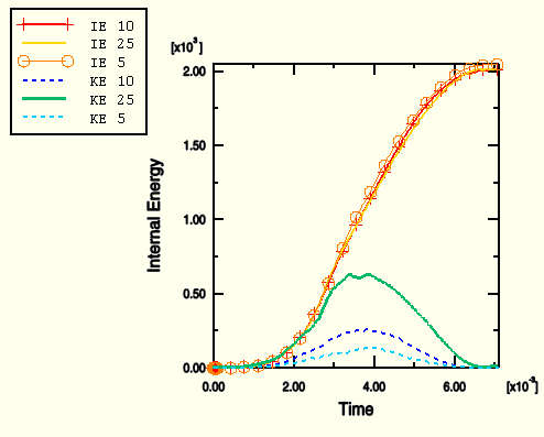
(mass scaling of 5), Figure 13–19 shows PEEQ for a speedup of ![]() (mass scaling of 10), and Figure 13–20 shows PEEQ for a speedup of 5 (mass scaling of 25). Figure 13–21 compares the internal and kinetic energy histories for each case of mass scaling. The mass scaling case using a factor of 5 yields results that are not significantly affected by the increased loading rate. The case with a mass scaling factor of 10 shows a high kinetic-to-internal energy ratio, yet the results seem reasonable when compared to those obtained with slower loading rates. Thus, this is likely close to the limit on how much this analysis can be sped up. The final case, with a mass scaling factor of 25, shows evidence of strong dynamic effects: the kinetic-to-internal energy ratio is quite high, and a comparison of the final deformed shapes among the three cases demonstrates that the deformed shape is significantly affected in the last case.
(mass scaling of 10), and Figure 13–20 shows PEEQ for a speedup of 5 (mass scaling of 25). Figure 13–21 compares the internal and kinetic energy histories for each case of mass scaling. The mass scaling case using a factor of 5 yields results that are not significantly affected by the increased loading rate. The case with a mass scaling factor of 10 shows a high kinetic-to-internal energy ratio, yet the results seem reasonable when compared to those obtained with slower loading rates. Thus, this is likely close to the limit on how much this analysis can be sped up. The final case, with a mass scaling factor of 25, shows evidence of strong dynamic effects: the kinetic-to-internal energy ratio is quite high, and a comparison of the final deformed shapes among the three cases demonstrates that the deformed shape is significantly affected in the last case.
Discussion of speedup methods
As the mass scaling increases, the solution time decreases. The quality of the results also decreases because dynamic effects become more prominent, but there is usually some level of scaling that improves the solution time without sacrificing the quality of the results. Clearly, a speedup of 5 is too great to produce quasi-static results for this analysis.
A smaller speedup, such as ![]() , does not alter the results significantly. These results would be adequate for most applications, including springback analyses. With a scaling factor of 10 the quality of the results begins to diminish, while the general magnitudes and trends of the results remain intact. Correspondingly, the ratio of kinetic energy to internal energy increases noticeably. The results for this case would be adequate for many applications but not for accurate springback analysis.
, does not alter the results significantly. These results would be adequate for most applications, including springback analyses. With a scaling factor of 10 the quality of the results begins to diminish, while the general magnitudes and trends of the results remain intact. Correspondingly, the ratio of kinetic energy to internal energy increases noticeably. The results for this case would be adequate for many applications but not for accurate springback analysis.
While it is possible to perform springback analyses within ABAQUS/Explicit, ABAQUS/Standard is much more efficient at solving springback analyses. Since springback analyses are simply static simulations without external loading or contact, ABAQUS/Standard can obtain a springback solution in just a few increments. Conversely, ABAQUS/Explicit must obtain a dynamic solution over a time period that is long enough for the solution to reach a steady state. For efficiency ABAQUS has the capability to transfer results back and forth between ABAQUS/Explicit and ABAQUS/Standard, allowing us to perform forming analyses in ABAQUS/Explicit and springback analyses in ABAQUS/Standard.
You will create a new model that imports the results from the analysis with a speedup of ![]() (mass scaling of 5) and perform a springback analysis. Thus, copy the Explicit model to a model named Import. Make all subsequent model changes to the Import model.
(mass scaling of 5) and perform a springback analysis. Thus, copy the Explicit model to a model named Import. Make all subsequent model changes to the Import model.
Since only the blank needs to be imported, begin by deleting the following features from the Import model:
Part instances Punch-1, Holder-1, and Die-1.
Sets RefDie, RefHolder, and RefPunch.
All surfaces.
All contact interactions and properties.
Both analysis steps.
Next, create a general static step named springback. Set the initial time increment to 0.1, and include the effects of geometric nonlinearity (note that the ABAQUS/Explicit analysis considered them; this is the default setting in ABAQUS/Explicit). Springback analyses can suffer from instabilities that adversely affect convergence. Thus, include automatic stabilization to prevent this problem. Use the default value for the dissipated energy fraction.
Next, define the initial state for the springback model based on the final state of the forming model.
To define an initial state:
In the Model Tree, double-click the Predefined Fields container. In the Create Predefined Field dialog box, select Initial as the step, Other as the category, and Initial State as the type. Click Continue.
In the viewport, select the blank as the instance to which the initial state will be assigned and click Done in the prompt area.
In the Edit Predefined Field dialog box that appears, enter the job name Forming-3--sqrt5. This corresponds to the job with a speedup of ![]() . Accept all other default settings, and click OK.
. Accept all other default settings, and click OK.
This will cause the state of the model—stresses, strains, etc.—to be imported. By not updating the reference configuration, the springback displacements will be referred to the original undeformed configuration. This will allow for continuity in the displacements in the event additional forming stages are required.
You must redefine the boundary conditions, which are not imported. Impose the same XSYMM-type displacement boundary conditions that were imposed in the ABAQUS/Explicit model on the set Center.
To remove rigid body motion, it is necessary to fix a single point in the blank , such as set MidLeft, in the 2-direction (in this way you impose no unnecessary constraints). Rather than apply a displacement boundary condition to this point, apply a zero-velocity boundary condition to fix this point at its final position at the end of the forming stage. This will allow the model to retain continuity in the blank location through any additional forming stages that may follow.
Create a new job named springback, and submit it for analysis.
Results of the springback analysis
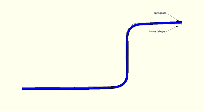
Figure 13–22 overlays (View![]() Overlay Plot) the deformed shape of the blank after the forming and springback stages (the forming stage corresponds to frame 0 in the output database file, while the springback stage corresponds to the final frame). The springback result is necessarily dependent on the accuracy of the forming stage preceding it. In fact, springback results are highly sensitive to errors in the forming stage, more sensitive than the results of the forming stage itself.
Overlay Plot) the deformed shape of the blank after the forming and springback stages (the forming stage corresponds to frame 0 in the output database file, while the springback stage corresponds to the final frame). The springback result is necessarily dependent on the accuracy of the forming stage preceding it. In fact, springback results are highly sensitive to errors in the forming stage, more sensitive than the results of the forming stage itself.
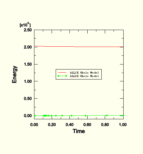
You should also plot the blank's internal energy ALLIE and compare it with the static stabilization energy ALLSD that is dissipated. The stabilization energy should be a small fraction of the internal energy to have confidence in the results. Figure 13–23 shows a plot of these two energies; the static stabilization energy is indeed small and, thus, has not significantly affected the results.