This simulation of the forming of a channel in a long metal sheet illustrates the use of rigid surfaces and some of the more complex techniques often required for a successful contact analysis in ABAQUS/Standard.
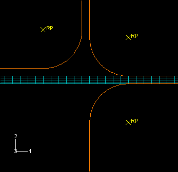
The problem consists of a strip of deformable material, called the blank, and the tools—the punch, die, and blank holder—that contact the blank. The tools can be modeled as rigid surfaces because they are much stiffer than the blank. Figure 12–14 shows the basic arrangement of the components.
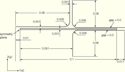
The blank is 1 mm thick and is squeezed between the blank holder and the die. The blank holder force is 440 kN. This force, in conjunction with the friction between the blank and blank holder and the blank and die, controls how the blank material is drawn into the die during the forming process. You have been asked to determine the forces acting on the punch during the forming process. You also must assess how well the channel is formed with these particular settings for the blank holder force and the coefficient of friction between the tools and blank.A two-dimensional, plane strain model will be used. The assumption that there is no strain in the out-of-plane direction of the model is valid if the structure is long in this direction. Only half of the channel needs to be modeled because the forming process is symmetric about a plane along the center of the channel.
The dimensions of the various components are shown in Figure 12–15.
Use ABAQUS/CAE to create the model. A Python script is provided in “Forming a channel,” Section A.12. When this script is run through ABAQUS/CAE, it creates the complete analysis model for this problem. Run this script if you encounter difficulties following the instructions given below or if you wish to check your work. Instructions on how to fetch and run the script are given in Appendix A, “Example Files.”
If you do not have access to ABAQUS/CAE or another preprocessor, the input file required for this problem can be created manually, as discussed in “Example: forming a channel,” Section 11.6 of Getting Started with ABAQUS/Standard: Keywords Version.
Part definition
Start ABAQUS/CAE (if you are not already running it). You will have to create four parts: a deformable part representing the blank and three rigid parts representing the tools.
Deformable blank
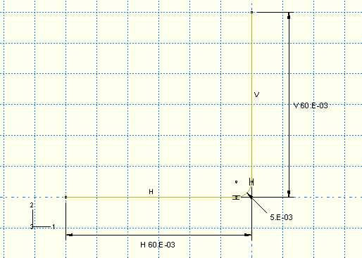
Create a two-dimensional, deformable solid part with a planar shell base feature to represent the deformable blank. Use an approximate part size of 0.25, and name the part Blank. To define the geometry, sketch a rectangle of arbitrary dimensions using the connected lines tool. Then, dimension the horizontal and vertical lengths of the rectangle, and edit the dimensions to define the part geometry precisely. The final sketch is shown in Figure 12–16.
Rigid tools
You must create a separate part for each rigid tool. Each of these parts will be created using very similar techniques so it is sufficient to consider the creation of only one of them (for example, the punch) in detail. Create a two-dimensional planar, analytical rigid part with a wire base feature to represent the rigid punch. Use an approximate part size of 0.25, and name the part Punch. Using the Create Lines and Create Fillet tools, sketch the geometry of the part. Create and edit the dimensions as necessary to define the geometry precisely. The final sketch is shown in Figure 12–17.
A rigid body reference point must be created. Exit the Sketcher when you are finished defining the part geometry to return to the Part module. From the main menu bar, select Tools![]() Reference Point. In the viewport, select the point at the center of the arc as the rigid body reference point.
Reference Point. In the viewport, select the point at the center of the arc as the rigid body reference point.
Next, create two additional analytical rigid parts named Holder and Die, representing the blank holder and rigid die, respectively. Since the parts are mirror images of each other, the easiest way to define the geometry of the new parts is to rotate the sketch created for the punch. (The Copy Part tool cannot be used to mirror analytical rigid parts.) For example, edit the punch feature, and save the sketch with the name Punch. Then, create a part named Holder, and add the Punch sketch to the part definition. Mirror the sketch about the vertical edge. Finally, create a part named Die, and add the Punch sketch to the part definition. In this case mirror the sketch twice: first about the vertical edge and then about the horizontal edge. Be sure to create a reference point at the center of the arc on each part.
Material and section properties
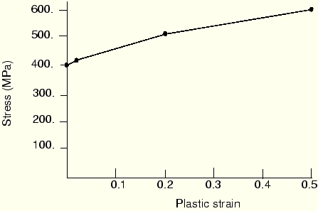
The blank is made from a high-strength steel (elastic modulus of 210.0 × 10⁹ Pa, ![]() = 0.3). Its inelastic stress-strain behavior is shown in Figure 12–18 and tabulated in Table 12–1. The material undergoes considerable work hardening as it deforms plastically. It is likely that plastic strains will be large in this analysis; therefore, hardening data are provided up to 50% plastic strain.
= 0.3). Its inelastic stress-strain behavior is shown in Figure 12–18 and tabulated in Table 12–1. The material undergoes considerable work hardening as it deforms plastically. It is likely that plastic strains will be large in this analysis; therefore, hardening data are provided up to 50% plastic strain.
Table 12–1 Yield stress–plastic strain data.
| Yield stress (Pa) | Plastic strain |
|---|---|
| 400.0E6 | 0.0 |
| 420.0E6 | 2.0E–2 |
| 500.0E6 | 20.0E–2 |
| 600.0E6 | 50.0E–2 |
Create a material named Steel with these properties. Create a homogeneous solid section named BlankSection that refers to the material Steel. Assign the section to the blank.
The blank is going to undergo significant rotation as it deforms. Reporting the values of stress and strain in a coordinate system that rotates with the blank's motion will make it much easier to interpret the results. Therefore, a local material coordinate system that is aligned initially with the global coordinate system but moves with the elements as they deform should be created. To do this, create a rectangular datum coordinate system using the Create Datum CSYS: 3 Points ![]() tool. From the main menu bar of the Property module, select Assign
tool. From the main menu bar of the Property module, select Assign![]() Material Orientation. Select the blank as the region to which the local material orientation will be assigned, and pick the datum coordinate system in the viewport as the CSYS (select Axis–1 and accept 0.0 for the additional rotation options).
Material Orientation. Select the blank as the region to which the local material orientation will be assigned, and pick the datum coordinate system in the viewport as the CSYS (select Axis–1 and accept 0.0 for the additional rotation options).
Assembling the parts
You will now create an assembly of part instances to define the analysis model. Begin by instancing the blank. Then, instance and position the rigid tools using the techniques described below.
To instance and position the punch:
In the Model Tree, double-click Instances underneath the Assembly container and select Punch as the part to instance.
Two-dimensional plane strain models must be defined in the global 1–2 plane. Therefore, do not rotate the parts after they have been instanced. You may, however, place the origin of the model at any convenient location. The 1-direction will be normal to the symmetry plane.
The bottom of the punch initially rests 0.001 m from the top of the blank, as indicated in Figure 12–15. From the main menu bar, select Constraint![]() Edge to Edge to position the punch vertically with respect to the blank.
Edge to Edge to position the punch vertically with respect to the blank.
Choose the horizontal edge of the punch as the straight edge of the movable instance and the edge on the top of the blank as the straight edge of the fixed instance.
Arrows appear on both instances. The punch will be moved so that its arrow points in the same direction as the arrow on the blank.
If necessary, click Flip in the prompt area to reverse the direction of the arrow on the punch so that both arrows point in the same direction; otherwise, the punch will be flipped. When both arrows point in the same direction, click OK.
Enter a distance of 0.001 m to specify the separation between the instances.
The punch is moved in the viewport to the specified location. Click the auto-fit tool ![]() so that the entire assembly is rescaled to fit in the viewport.
so that the entire assembly is rescaled to fit in the viewport.
The vertical edge of the punch is 0.05 m from the left edge of the blank, as shown in Figure 12–15. Define another Edge to Edge constraint to position the punch horizontally with respect to the blank.
Select the vertical edge of the punch as the straight edge of the movable instance and the left edge of the blank as the straight edge of the fixed instance. Flip the arrow on the punch if necessary so that both arrows point in the same direction. Enter a distance of –0.05 m to specify the separation between the edges. (A negative distance is used since the offset is applied in the direction of the edge normal. The edge normal points away from the edge of the blank.)
Now that you have positioned the punch relative to the blank, check to make sure that the left end of the punch extends beyond the left edge of the blank. This is necessary to prevent any nodes associated with the blank from “falling off” the rigid surface associated with the punch during the contact calculations. If necessary, return to the Part module and edit the part definition to satisfy this requirement.
To instance and position the blank holder:
The procedure for instancing and positioning the holder is very similar to that used to instance and position the punch. Referring to Figure 12–15, we see that the holder is initially positioned so that its horizontal edge is offset a distance of 0.0 m from the top edge of the blank and its vertical edge is offset a distance of 0.001 m from the vertical edge of the punch. Define the necessary Edge to Edge constraints to position the blank holder. Remember to flip the directions of the arrows as necessary, and make sure the right end of the holder extends beyond the right edge of the blank. If necessary, return to the Part module and edit the part definition.
To instance and position the die:
The procedure for instancing and positioning the die is very similar to that used to instance and position the other tools. Referring to Figure 12–15, we see that the die is initially positioned so that its horizontal edge is offset a distance of 0.0 m from the bottom edge of the blank and its vertical edge is offset a distance of 0.051 m from the left edge of the blank. Define the necessary Edge to Edge constraints to position the die. Remember to flip the directions of the arrows as necessary, and make sure the right end of the die extends beyond the right edge of the blank. If necessary, return to the Part module and edit the part definition.
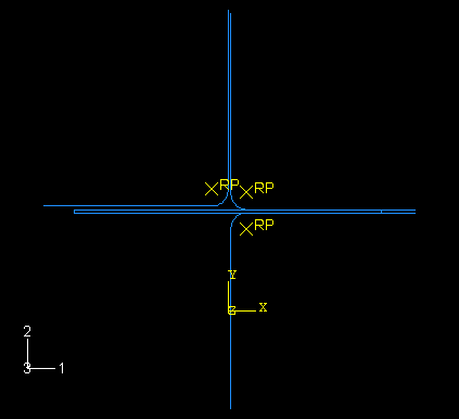
The final assembly is shown in Figure 12–19.
Geometry sets
At this point it is convenient to create the geometry sets that will be used to specify loads and boundary conditions and to restrict data output. Six sets should be created: one at each rigid body reference point, one at the symmetry plane of the blank, and one at each end of the blank midplane. The last two sets require that a vertex first exist at these locations; an edge partition can be performed to satisfy this requirement.
Begin by partitioning the vertical edges of the blank in half using the procedure described below.
To create vertices on the blank midplane:
In the Model Tree, double-click the part named Blank underneath the Parts container. Partition the left and right vertical edges of the blank using the Partition Edge: Enter Parameter tool. For each edge, specify a normalized edge parameter of 0.5 to partition the edge in half.
Each vertical edge of the blank now has a vertex located on the blank midplane.
Double-click the Sets item underneath the Assembly container to create the following geometry sets:
RefPunch at the punch rigid body reference point.
RefHolder at the holder rigid body reference point.
RefDie at the die rigid body reference point.
Center at the left vertical edges (symmetry plane) of the blank.
MidLeft at the left midplane vertex of the blank.
MidRight at the right midplane vertex of the blank.
Defining steps and output requests
There are two major sources of difficulty in ABAQUS/Standard contact analyses: rigid body motion of the components before contact conditions constrain them and sudden changes in contact conditions, which lead to severe discontinuity iterations as ABAQUS/Standard tries to establish the exact condition of all contact surfaces. Therefore, wherever possible, take precautions to avoid these situations.
Removing rigid body motion is not particularly difficult. Simply ensure that there are enough constraints to prevent all rigid body motions of all the components in the model. This may mean using boundary conditions initially to get the components into contact, instead of applying loads directly. Using this approach may require more steps than originally anticipated, but the solution of the problem should proceed more smoothly.
Unless a dynamic impact event is being simulated, always try to establish contact between components in a reasonably smooth manner, avoiding large overclosures and rapid changes in contact pressure. Again, this usually means adding additional steps to the analysis to move components into contact before fully loading them. This approach, although requiring more steps, will minimize convergence difficulties and, therefore, make the solution far more efficient. With these points in mind, we can now define the steps for this example.
The simulation will consist of five steps. Since the simulation involves material, geometric, and boundary nonlinearities, general steps must be used. In addition, the forming process is quasi-static; thus, we can ignore inertia effects throughout the simulation. A brief summary of each step (including the details of its purpose, definition, and associated output requests) is given below. However, the details concerning how the loads and boundary conditions are applied are discussed later.
Step 1
This step is intended to establish firm contact between the blank and the blank holder. In this step the endpoints of the midplane of the blank will be fixed in the vertical direction to prevent the blank from moving initially, and the blank holder will be pushed down onto the blank using a displacement boundary condition.
Given the quasi-static nature of the problem and the fact that nonlinear response will be considered, create a static, general step named Establish contact I after the Initial step. Enter the following description for the step: Push the blank holder and die together; and include the effects of geometric nonlinearity. The step should complete in one increment, so set the initial time increment and the total time to be equal (for example, 1.0). To limit the amount of output, write the preselected field output only at the end of the step. In addition, you can delete the history output request for this step. Output for variables that you need to track using history data can be requested, when needed, at a later stage in the analysis. In addition, write contact diagnostics to the message file (Output![]() Diagnostic Print).
Diagnostic Print).
Step 2
Since contact was established between the blank and the blank holder and die in the previous step, the constraint on the right end of the blank midplane is no longer necessary and will be removed in a second static, general step. Name the second step Remove right constraint, and insert it after the Establish contact I step. Enter the following description for the step: Remove the middle constraint at right. Since the previous step considers the effects of geometric nonlinearity, these effects will be included automatically in this and all subsequent general steps and cannot be removed. This step should also complete in a single increment because the only change being made to the model is the removal of the vertical constraints on the blank; therefore, set the initial time increment and the total time to be equal (again, set them equal to 1.0). The field output request specified in the previous step will be propagated to this step. You should request contact diagnostic output for Step 2 as well.
Step 3
The magnitude of the blank holder force is a controlling factor in many forming processes; therefore, it needs to be introduced as a variable load in the analysis. In this step the boundary condition used to move the blank holder down will be replaced with a force.
Create a third static, general step named Holder force, and insert it after the Remove right constraint step. Enter the following description for the step: Apply prescribed force on blank holder. This step will also complete in a single increment; therefore, again set the initial time increment to be equal to the total time period. Request contact diagnostic output for this step.
Step 4
At the beginning of the analysis the punch and the blank are separated to avoid any interference while contact is established between the blank and the die and blank holder. In this step the punch will be moved down in the 2-direction just enough to achieve contact with the blank. In addition, the vertical constraint on the left end of the blank midplane will be removed; and a small pressure will be applied to the top surface of the blank to pull it onto the surface of the punch.
Create a fourth static, general step named Establish contact II, and insert it after the Holder force step. Enter the following description for the step: Move the punch down a little while applying a small pressure to blank top. Set the initial time increment to 10% of the total time since the contact condition may be harder to establish in this step. Request contact diagnostic output for Step 4. In addition, request that the reaction forces at the punch reference point (geometry set RefPunch) be written every increment as history data.
Step 5
In the fifth and final step the pressure load applied to the blank will be removed, and the punch will be moved down to complete the forming operation.
Create a fifth static, general step named Move punch, and insert it after the Establish contact II step. Enter the following description for the step: Full extent. Because of the frictional sliding, the changing contact conditions, and the inelastic material behavior, there is significant nonlinearity in this step; therefore, set the maximum number of increments to a large value (for example, 1000). Set the initial time increment to 0.0001, the total time period to 1.0, and the minimum time increment to 1e–06. With these settings ABAQUS/Standard can take smaller time increments during the highly nonlinear parts of the response without terminating the analysis. Specify that the preselected field output be written every 20 increments for this step. Your history output request for the punch reaction forces from the previous step will be propagated to this step. Remember to specify the contact diagnostics output request as well. In addition, request that the restart file be written every 200 increments for Step 5.
Monitoring the value of a degree of freedom
You can request that ABAQUS monitor the value of a degree of freedom at one selected point. The value of the degree of freedom is shown in the Job Monitor and is written at every increment to the status (.sta) file and at specific increments during the course of an analysis to the message (.msg) file. In addition, a plot of the degree of freedom value over time appears in a new viewport that is generated automatically when you submit the analysis. You can use this information to monitor the progress of the solution.
In this model you will monitor the vertical displacement (degree of freedom 2) of the punch's reference node throughout each step. Before proceeding, make the first analysis step (Establish contact I) active by selecting it from the Step list located under the toolbar. The monitor definition applied for this step will be propagated automatically to all the subsequent steps.
To select a degree of freedom to monitor:
From the main menu bar of the Step module, select Output![]() DOF Monitor.
DOF Monitor.
The DOF Monitor dialog box appears.
Toggle Monitor a degree of freedom throughout the analysis.
Click Edit to select the region. In the prompt area, click Points. In the Region Selection dialog box that appears, select RefPunch; and click Continue.
In the Degree of freedom text field, enter 2.
Accept the default frequency (every increment) at which this information will be written to the message file.
Click OK to exit the DOF Monitor dialog box.
Defining contact interactions
Contact must be defined between the top of the blank and the punch, the top of the blank and the blank holder, and the bottom of the blank and the die. The rigid surface must be the master surface in each of these contact interactions. Each contact interaction must refer to a contact interaction property that governs the interaction behavior.
In this example we assume that the friction coefficient is zero between the blank and the punch. The friction coefficient between the blank and the other two tools is assumed to be 0.1. Therefore, two contact interaction properties must be defined: one with friction and one without.
Define the following surfaces: BlankTop on the top edge of the blank; BlankBot on the bottom edge of the blank; DieSurf on the side of the die that faces the blank; HolderSurf on the side of the holder that faces the blank; and PunchSurf on the side of the punch that faces the blank.
Now define two contact interaction properties. (In the Model Tree, double-click the Interaction Properties container to create a contact property.) Name the first one NoFric; since frictionless contact is the default in ABAQUS, accept the default property settings for the tangential behavior (select Mechanical![]() Tangential Behavior in the Edit Contact Property dialog box). The second property should be named Fric. For this property use the Penalty friction formulation with a friction coefficient of 0.1.
Tangential Behavior in the Edit Contact Property dialog box). The second property should be named Fric. For this property use the Penalty friction formulation with a friction coefficient of 0.1.
Finally, define the interactions between the surfaces and refer to the appropriate contact interaction property for each definition. (In the Model Tree, double-click the Interactions container to define a contact interaction.) In all cases define the interactions in the Initial step and use the default finite-sliding formulation (Surface-to-surface contact (Standard)). The following interactions should be defined:
Die-Blank between surfaces DieSurf (master) and BlankBot (slave) referring to the Fric contact interaction property.
Holder-Blank between surfaces HolderSurf (master) and BlankTop (slave) referring to the Fric contact interaction property.
Punch-Blank between surfaces PunchSurf (master) and BlankTop (slave) referring to the NoFric contact interaction property.
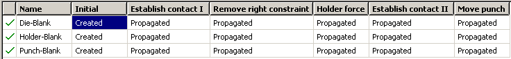
The Interaction Manager shows that each interaction has been created in the Initial step and propagated to all subsequent steps, as shown in Figure 12–20.
Boundary conditions for Step 1
Recall that the first stage of the process is to hold the blank between the blank holder and the die. At the start of the first increment of the analysis contact may not be fully established between the various components, even though their surfaces are coincident initially. Problems can occur when contact is not fully established: components may undergo rigid body motion; or the contact status may oscillate between open and closed, which is known as chattering. Chattering is especially common in contact analyses with multiple components.
To avoid rigid body motions and chattering in this simulation, the endpoints of the midplane of the blank will be fixed in the vertical direction to prevent the blank from moving initially. These points are used because constraints should not be applied to regions that are also part of a contact surface. If a contact region is constrained by a boundary condition in the direction that contact occurs, there will be two constraints applied to a single degree of freedom. This can cause numerical problems, and ABAQUS/Standard may issue a zero pivot warning message in the message file.
One method of establishing contact is to apply a force to the blank holder. However, the blank holder may undergo rigid body motion in the vertical direction because contact between the blank holder and the blank may not be fully established. Therefore, it is better to move the blank holder by means of an applied displacement. This ensures firm contact between these two surfaces. In addition, move the die slightly upward to establish firm contact between it and the blank. The magnitude of the applied displacement should be large enough so that firm contact is established yet small enough so that plastic yielding does not occur.
Constrain the blank holder and die in degrees of freedom 1 and 6, where degree of freedom 6 is the rotation in the plane of the model. All of the boundary conditions for the rigid surfaces are applied to their respective rigid body reference nodes. Constrain the punch completely, and apply symmetric boundary constraints on the region of the blank lying on the symmetry plane (geometry set Center).
Table 12–2 summarizes the boundary conditions applied in this step:
Boundary conditions for Step 2
Now that contact between the blank and the blank holder and die has been established, the blank is fully constrained in the 2-direction. Therefore, deactivate the boundary condition on the right side of the midplane of the blank (it is no longer necessary). To do this, open the Boundary Condition Manager and click the cell under Remove right constraint in the row for boundary condition MidRightBC. Click Deactivate on the right side of the dialog box.
Loading and boundary conditions for Step 3
In this step the boundary condition used to move the blank holder down should be removed and replaced with a concentrated force. There should be no problems replacing the applied displacement on the blank holder with a force because there is firm contact between the blank holder and the blank. In this simulation the required blank holder force is 440 kN. Generally, care should be taken to ensure that the newly applied force is of the same order as the reaction force generated from the boundary condition so that the contact condition does not change significantly.
Using the Boundary Condition Manager, edit the RefHolderBC boundary condition in Step 3 to remove the constraint on U2.
Create a mechanical concentrated force in this step named RefHolderForce. Apply the load to set RefHolder in step Holder force. Specify a magnitude of –440.E3 for CF2.
Loading and boundary conditions for Step 4
In this step the punch must be moved down in the 2-direction just enough to achieve contact with the blank. The vertical constraint on set MidLeft should be removed, and a small pressure should be applied to the top surface of the blank to pull it onto the surface of the punch.
Using the Boundary Condition Manager, deactivate the MidLeftBC boundary condition in Step 4 and change the RefPunchBC boundary condition to specify a value of –0.001 for U2.
It can be difficult to choose the proper magnitude of pressure to apply. In this analysis you should use a pressure magnitude (1000 Pa) that produces a force on the blank that is three orders of magnitude lower than the blank holder force. A positive pressure acts into the surface; however, in this simulation you want the pressure to act out of the surface, so use a negative pressure. This technique is used to prevent chattering of the BlankTop and Punch surfaces.
Create a mechanical pressure load named Small pressure. Apply the load to the surface BlankTop in step Establish contact II. Specify a magnitude of -1000.0.
Loading and boundary conditions for Step 5
In this step remove the pressure load applied to surface BlankTop, and move the punch down to complete the forming operation. When a pressure load is removed in a static analysis, the magnitude is ramped down to zero over the duration of the step. Therefore, the pressure will continue to pull on the surface BlankTop and hold it tightly against the punch, maintaining contact between the surfaces, particularly in the early part of the step. This helps prevent chattering between the punch and the blank at the beginning of the forming process. As long as the force created by the pressure is small compared to the force required to move the punch, it will have little effect on the solution. Using the Load Manager, deactivate the Small pressure load in this step. Using the Boundary Condition Manager, edit the RefPunchBC boundary condition to specify a value of –0.031 for U2. This represents the total displacement of the punch, accounting for the initial offset of 0.001 m.
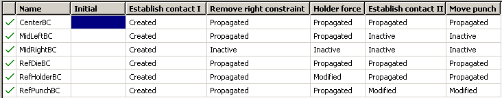
For reference, the contents of the Boundary Condition Manager appear in Figure 12–21.
Before continuing, change the name of your model to Standard.
Mesh creation and job definition
You should consider the type of element you will use before you design your mesh. When choosing an element type, you must consider several aspects of your model such as the model's geometry, the type of deformation that will be seen, the loads being applied, etc. The following points are important to consider in this simulation:
The contact between surfaces. Whenever possible, first-order elements (with the exception of tetrahedral elements) should be used for contact simulations. When using tetrahedral elements, modified second-order tetrahedral elements should be used for contact simulations.
Significant bending of the blank is expected under the applied loading. Fully integrated first-order elements exhibit shear locking when subjected to bending deformation. Therefore, either reduced-integration or incompatible mode elements should be used.
Create a job named Channel. Give the job the following description: Analysis of the forming of a channel. Save your model to a model database file, and submit the job for analysis. Monitor the solution progress, correct any modeling errors that are detected, and investigate the cause of any warning messages.
Once the analysis is underway, an X–Y plot of the values of the degree of freedom that you selected to monitor (the punch's vertical displacement) appears in a separate viewport. From the main menu bar, select Viewport![]() Job Monitor: Channel to follow the progression of the punch's displacement in the 2-direction over time as the analysis runs.
Job Monitor: Channel to follow the progression of the punch's displacement in the 2-direction over time as the analysis runs.
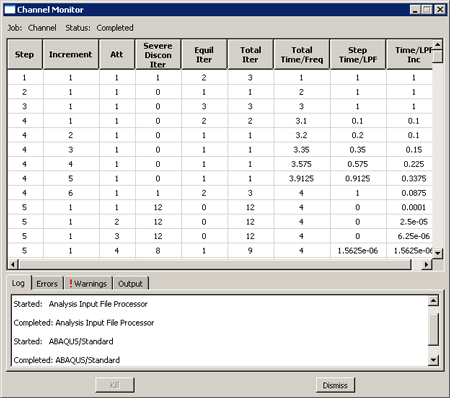
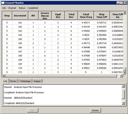
This analysis should take approximately 170 increments to complete. The top of the Job Monitor is shown in Figure 12–23.
The value of the punch displacement appears in the Output tabbed page. This simulation contains many severe discontinuity iterations. ABAQUS/Standard has a very difficult time determining the contact state in the first increment of Step 5. It needs four attempts before it finds the proper configuration of the PunchSurf and BlankTop surfaces. Once it finds the correct configuration, ABAQUS/Standard needs only a single iteration to achieve equilibrium. After this difficult start, ABAQUS/Standard quickly increases the increment size to a more reasonable value. The end of the Job Monitor is shown in Figure 12–24.Contact analyses are generally more difficult to complete than just about any other type of simulation in ABAQUS/Standard. Therefore, it is important to understand all of the options available to help you with contact analyses.
If a contact analysis runs into difficulty, the first thing to check is whether the contact surfaces are defined correctly. The easiest way to do this is to run a datacheck analysis and plot the surface normals in the Visualization module. You can plot all of the normals, for both surfaces and structural elements, on either the deformed or the undeformed plots. Use the Normals options in the Common Plot Options dialog box to do this, and confirm that the surface normals are in the correct directions.
ABAQUS/Standard may still have some problems with contact simulations, even when the contact surfaces are all defined correctly. One reason for these problems may be the default convergence tolerances and limits on the number of iterations: they are quite rigorous. In contact analyses it is sometimes better to allow ABAQUS/Standard to iterate a few more times rather than abandon the increment and try again. This is why ABAQUS/Standard makes the distinction between severe discontinuity iterations and equilibrium iterations during the simulation.
The diagnostic contact information is essential for almost every contact analysis. This information can be vital for spotting mistakes or problems. For example, chattering can be spotted because the same slave node will be seen to be involved in all of the severe discontinuity iterations. If you see this, you will have to modify the mesh in the region around that node or add constraints to the model. Contact diagnostic information can also identify regions where only a single slave node is interacting with a surface. This is a very unstable situation and can cause convergence problems. Again, you should modify the model to increase the number of elements in such regions.
Contact diagnostics
To illustrate how to interpret the contact diagnostic information in ABAQUS/CAE, consider the iterations in the sixth increment of the fourth step. As shown in Figure 12–23, this is one of the first increments in which severe discontinuity iterations are required. ABAQUS/Standard requires one iteration to establish the correct contact conditions in the model; i.e., whether or not the punch was contacting the blank. The second iteration does not produce any changes in the model's contact condition, so ABAQUS/Standard checks the force equilibrium. One additional iteration is required to converge on static equilibrium. Thus, once ABAQUS/Standard determines the correct contact state, it can easily find the equilibrium solution.
To further investigate the behavior of the model in this increment, look at the visual diagnostic information available in ABAQUS/CAE. The diagnostic information written to the output database file provides detailed information about the changes in the model's contact conditions. For example, the node number and location in the model of every slave node whose contact status changes in a severe discontinuity iteration, as well as the contact interaction to which it belongs, can be obtained using the visual diagnostics tool.
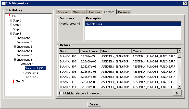
Enter the Visualization module, and open the file Channel.odb to look at the contact diagnostics information. In the first severe discontinuity iteration of the fourth step, 46 nodes on the blank experience contact overclosure, indicating that their contact status should be changed. This can be seen in the Contact tabbed page of the Job Diagnostics dialog box (see Figure 12–25). To see where the nodes are located on the model, toggle on Highlight selections in viewport.
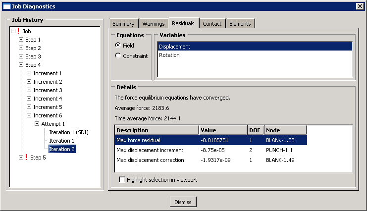
ABAQUS/Standard removes the contact constraints from these nodes and performs another iteration; this time ABAQUS/Standard detects no changes in the contact state and, therefore, carries out the normal equilibrium convergence checks. The solution in this iteration does not satisfy the force residual tolerance check, so another iteration is performed. This time, the force residual tolerance check is satisfied and the displacement correction is acceptable relative to the largest displacement increment, as shown in Figure 12–26. Thus, the second equilibrium iteration produces a converged solution for this increment.
In the Visualization module, examine the deformation of the blank.
Deformed model shape and contour plots
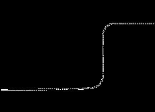
The basic result of this simulation is the deformation of the blank and the plastic strain caused by the forming process. We can plot the deformed model shape and the plastic strain, as described below.
To plot the deformed model shape:
Plot the deformed model shape. You can remove the die and the punch from the display and visualize just the blank.
In the Results Tree, expand the Instances container underneath the output database file named Channel.odb.
From the list of available part instances, select BLANK-1. Click mouse button 3, and select Replace from the menu that appears to replace the current display group with the selected elements. Click ![]() , if necessary, to fit the model in the viewport.
, if necessary, to fit the model in the viewport.
The resulting plot is shown in Figure 12–27.
To plot the contours of equivalent plastic strain:
From the main menu bar, select Plot![]() Contours
Contours![]() On Deformed Shape; or click the
On Deformed Shape; or click the ![]() tool from the toolbox to display contours of Mises stress.
tool from the toolbox to display contours of Mises stress.
Open the Contour Plot Options dialog box.
Drag the Contour Intervals slider to change the number of contour intervals to 7.
Click OK to apply these settings.
From the main menu bar, select Result![]() Field Output.
Field Output.
The Field Output dialog box appears.
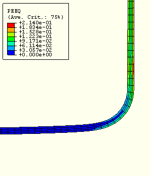
Select PEEQ from the Output Variable list.
PEEQ is an integrated measure of plastic strain. A non-integrated measure of plastic strain is PEMAG. PEEQ and PEMAG are equal for proportional loading.
Click OK to apply these settings. Use the ![]() tool to zoom into any region of interest in the blank, as shown in Figure 12–28.
tool to zoom into any region of interest in the blank, as shown in Figure 12–28.
The maximum plastic strain is 21.4%. Compare this with the failure strain of the material to determine if the material will tear during the forming process.
History plots of the reaction forces on the blank and punch
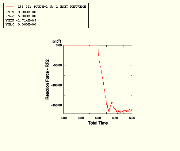
It is important to check that the force required to push the punch into the blank is much larger than the force created by the pressure applied to the surface of the blank. The force on the blank from the applied pressure is approximately 100 N (1000 Pa × 0.1 m × 1.0 m) at the start of Step 5. The solid line in Figure 12–29 shows the variation of the reaction force RF2 at the punch's rigid body reference node.
To create a history plot of the reaction force:
In the Results Tree, expand the History Output container. Double-click Reaction force: RF1 PI: PUNCH-1 Node xxx in NSET REFPUNCH.
A history plot of the reaction force in the 1-direction appears.
Select and plot Reaction force: RF2 PI: PUNCH-1 Node xxx in NSET REFPUNCH.
Open the XY Plot Options dialog box to label the axes.
Click the Titles tab, and select User-specified from the Title source lists for the X-Axis and Y-Axis labels.
Specify Reaction Force - RF2 as the Y-Axis label, and specify Total Time as the X-Axis label.
Click OK to apply the settings and to close the dialog box.
From the main menu bar, select Viewport![]() Viewport Annotation Options, click the Legend tab in the dialog box that appears, and toggle on Show min/max values.
Viewport Annotation Options, click the Legend tab in the dialog box that appears, and toggle on Show min/max values.
Click OK to apply your change and to close the dialog box.
The punch force, shown in Figure 12–29, rapidly increases to about 160 kN during Step 5, which runs from a total time of 4.0 to 5.0. The punch force clearly is much larger than the force (100 N) created by the pressure load.
Plotting contours on surfaces
ABAQUS/CAE includes a number of features designed specifically for postprocessing contact analyses. Within the Visualization module, the Display Group feature can be used to collect surfaces into display groups, similar to element and node sets.
To display contact surface normal vectors:
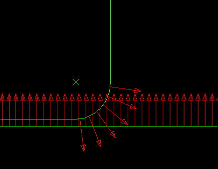
Plot the undeformed model shape.
In the Results Tree, expand the Surface Sets container. Select the surfaces named BLANKTOP and PUNCH-1.PUNCHSURF. Click mouse button 3, and select Replace from the menu that appears.
Using the Common Plot Options dialog box, turn on the display of the normal vectors (On surfaces) and set the length of the vector arrows to Short.
Use the ![]() tool, if necessary, to zoom into any region of interest, as shown in Figure 12–30.
tool, if necessary, to zoom into any region of interest, as shown in Figure 12–30.
To contour the contact pressure:
Plot the contours of plastic strain again.
From the main menu bar, select Result![]() Field Output.
Field Output.
The Field Output dialog box appears.
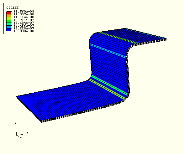
Select CPRESS from the Output Variable list.
Click OK to apply these settings.
Remove the PUNCH-1.PUNCHSURF surface from your display group.
To better visualize contours of surface-based variables in two-dimensional models, you can extrude the plane strain elements to construct the equivalent three-dimensional view. You can sweep axisymmetric elements in a similar fashion.
From the main menu bar, select View![]() ODB Display Options.
ODB Display Options.
The ODB Display Options dialog box appears.
Select the Sweep/Extrude tab to access the Sweep/Extrude options.
In the Extrude region of the dialog box, toggle on Extrude elements; and set the Depth to 0.05 to extrude the model for the purpose of displaying contours.
Click OK to apply these settings.
Rotate the model using the ![]() tool to display the model from a suitable view, such as the one shown in Figure 12–31.
tool to display the model from a suitable view, such as the one shown in Figure 12–31.