The previous example illustrated some of the convergence difficulties that may be encountered when solving problems involving a nonlinear material response using implicit methods. We will now focus on solving a problem involving plasticity using explicit dynamics. As will become evident shortly, convergence difficulties are not an issue in this case since iteration is not required for explicit methods.
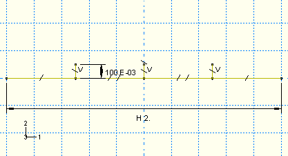
In this example you will assess the response of a stiffened square plate subjected to a blast loading in ABAQUS/Explicit. The plate is firmly clamped on all four sides and has three equally spaced stiffeners welded to it. The plate is constructed of 25 mm thick steel and is 2 m square. The stiffeners are made from 12.5 mm thick plate and have a depth of 100 mm. Figure 10–25 shows the plate geometry and material properties in more detail. Since the plate thickness is significantly smaller than any other global dimensions, shell elements can be used to model the plate.
The purpose of this example is to determine the response of the plate and to see how it changes as the sophistication of the material model increases. Initially, we analyze the behavior with the standard elastic-plastic material model. Subsequently, we study the effects of including material damping and rate-dependent material properties.
Use ABAQUS/CAE to create a three-dimensional model of the stiffened plate. A Python script is provided in “Blast loading on a stiffened plate,” Section A.9. When this script is run through ABAQUS/CAE, it creates the complete analysis model for this problem. Run this script if you encounter difficulties following the instructions given below or if you wish to check your work. Instructions on how to fetch and run the script are given in Appendix A, “Example Files.”
If you do not have access to ABAQUS/CAE or another preprocessor, the input file required for this problem can be created manually, as discussed in “Example: blast loading on a stiffened plate,” Section 5.3 of Getting Started with ABAQUS/Explicit: Keywords Version.
Defining the model geometry
Create a three-dimensional, deformable part with an extruded shell base feature to represent the plate. Use an approximate part size of 5.0, and name the part Plate. A suggested approach for creating the part geometry shown in Figure 10–26 is summarized in the following procedure:
To create the stiffened plate geometry:
To define the plate geometry, use the Create Lines: Connected tool to sketch an arbitrary horizontal line.
To define the stiffener geometry, add three vertical lines extending up from the plate. The horizontal position of these lines is arbitrary at this stage, but their endpoints must snap to the horizontal line.
Constrain the three vertical lines so they are of equal length, and dimension one of them so that it is 0.1 m long.
Split the plate at the points where it intersects the stiffeners.
Dimension the horizontal distance between the plate endpoints, and set the value to 2.0 m.
Apply equal length constraints to the four horizontal segments of the line.
The final part sketch is shown in Figure 10–26.
Extrude the sketch to a depth of 2.0 m to create the plate.
Defining the material properties
Define the material and section properties for the plate and the stiffeners.
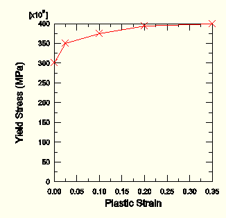
Create a material named Steel with a mass density of 7800 kg/m3, a Young's modulus of 210.0E9 Pa, and a Poisson's ratio of 0.3. At this stage we do not know whether there will be any plastic deformation, but we know the value of the yield stress and the details of the post-yield behavior for this steel. We will include this information in the material definition. The initial yield stress is 300 MPa, and the yield stress increases to 400 MPa at a plastic strain of 35%. To define the plastic material properties, enter the yield stress and plastic strain data shown in Figure 10–25. The plasticity stress-strain curve is shown in Figure 10–27.
During the analysis ABAQUS calculates values of yield stress from the current values of plastic strain. As discussed earlier, the process of lookup and interpolation is most efficient when the stress-strain data are at equally spaced values of plastic strain. To avoid having the user input regular data, ABAQUS/Explicit automatically regularizes the data. In this case the data are regularized by ABAQUS/Explicit by expanding the data to 15 equally spaced points with increments of 0.025.
To illustrate the error message that is produced when ABAQUS/Explicit cannot regularize the material data, you could set the regularization tolerance to 0.001 (in the Edit Material dialog box, select General![]() Regularization) and include one additional data pair, as shown in Table 10–2.
Regularization) and include one additional data pair, as shown in Table 10–2.
Table 10–2 Modified plasticity data.
| Yield Stress (Pa) | Plastic Strain |
|---|---|
| 300.0E6 | 0.000 |
| 349.0E6 | 0.001 |
| 350.0E6 | 0.025 |
| 375.0E6 | 0.100 |
| 394.0E6 | 0.200 |
| 400.0E6 | 0.350 |
 ***ERROR: Failed to regularize material data. Please check
 your input data to see if they meet both criteria as
 explained in the "MATERIAL DEFINITION" section of the
 ABAQUS Analysis User's Manual. In general, regularization is
 more difficult if the smallest interval defined by the user
 is small compared to the range of the independent variable.
Before continuing, set the regularization tolerance back to the default value (0.03) and remove the additional pair of data points.
Creating and assigning section properties
Create two homogeneous shell section properties, each referring to the steel material definition but specifying different shell thicknesses. Name the first shell section property PlateSection, select Steel as the material, and specify 0.025 m as the value for the Shell thickness. Name the second shell section property StiffSection, select Steel as the material, and specify 0.0125 m as the value for the Shell thickness.
Assign the StiffSection definition to the stiffeners (use [Shift]+Click to select multiple regions in the viewport).
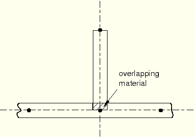
Before assigning the PlateSection definition to the plate, consider the following. If the plate and the stiffeners are joined directly at their midsurfaces (this is the default behavior), an area of material overlap will occur, as shown in Figure 10–28.
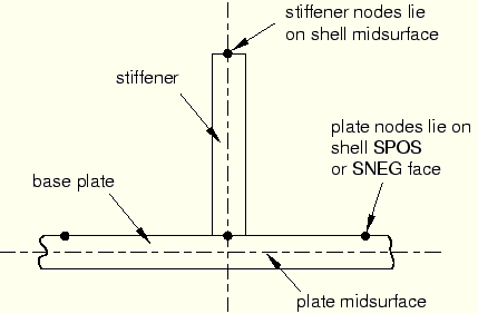
Although the thicknesses of the plate and stiffener are small in comparison to the overall dimensions of the structure (so that this overlapping material and the extra stiffness it creates would have little effect on the analysis results), a more precise model can be created by offsetting the plate reference surface from its midsurface. This technique allows the stiffeners to butt up against the plate without overlapping any material with the plate, as shown in Figure 10–29.To determine whether to offset the plate reference surface to its positive (SPOS) or negative (SNEG) side, query the shell normals (Tools![]() Query) and note the color of the side of the plate facing the stiffeners (brown is the positive side; purple is the negative side). If necessary, flip the plate normals (Assign
Query) and note the color of the side of the plate facing the stiffeners (brown is the positive side; purple is the negative side). If necessary, flip the plate normals (Assign![]() Normal) so that its segments have consistent normals. Then assign the PlateSection definition to the regions of the plate. In the Edit Section Assignment dialog box, toggle on Offset and enter 0.5 as the value of the offset if the brown (positive) side of the plate faces the stiffeners and –0.5 if the purple (negative) side faces the stiffeners.
Normal) so that its segments have consistent normals. Then assign the PlateSection definition to the regions of the plate. In the Edit Section Assignment dialog box, toggle on Offset and enter 0.5 as the value of the offset if the brown (positive) side of the plate faces the stiffeners and –0.5 if the purple (negative) side faces the stiffeners.
Note: Setting the offset value to 0.5 offsets the reference surface of the plate one half of the shell thickness away from its midsurface in the direction of the positive shell normal; setting the offset value to –0.5 offsets the reference surface the same distance but in the opposite direction.
Creating an assembly
Create a dependent instance of the plate. Use the default rectangular coordinate system, with the plate lying in the 1–3 plane.
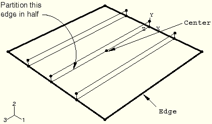
At this point, it is convenient to create the geometry sets that will be used to specify boundary conditions and output requests. Create one set named Edge for the plate edges and one set named Center at the center of the intersection of the plate and the middle stiffener, as shown in Figure 10–30. To create the set Center, you need to partition the edge of the original part in half using the Partition Edge: Enter Parameter ![]() tool.
tool.
Defining steps and output requests
Create a single dynamic, explicit step. Name the step Blast, and specify the following step description: Apply blast loading. Enter a value of 50E-3 s for the time period of the step.
In general, you should try to limit the number of frames written during the analysis to keep the size of the output database file reasonable. In this analysis saving information every 2 ms should provide sufficient detail to study the response of the structure. Edit the default output request F-Output-1, and set the number of intervals during the step at which preselected field data are saved to 25. This ensures that the selected data are written every 2 ms since the total time for the step is 50 ms.
A more detailed set of output for selected regions of the model can be saved as history output. Edit the default history output request H-Output-1 to write the whole model energies (selected by default) as well as displacement data for the center of the plate as history data to the output database file at 500 points during the analysis (i.e., every 1.0E–4 s of simulation time).
Create a history output request named Center-U2 for the step Blast. Select Center as the output domain, and select U2 as the translation output variable. Enter 500 as the number of intervals at which the output will be saved during the analysis.
Prescribing boundary conditions and loads
Next, define the boundary conditions used in this analysis. Create a Symmetry/Antisymmetry/Encastre mechanical boundary condition in step Blast named Fix edges. Apply the boundary condition to the edges of the plate using the geometry set Edge, and specify ENCASTRE (U1 = U2 = U3 = UR1 = UR2 = UR3 = 0) to fully constrain the set.
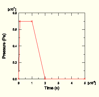
The plate will be subjected to a load that varies with time: the pressure increases rapidly from zero at the start of the analysis to its maximum of 7.0 × 10⁵ N in 1 ms, at which point it remains constant for 9 ms before dropping back to zero in another 10 ms. It then remains at zero for the remainder of the analysis. See Figure 10–31 for details.
Define a tabular amplitude curve named Blast. Enter the amplitude data given in Table 10–3, and specify a smoothing parameter of 0.0.
Next, define the pressure loading. Since the magnitude of the load will be defined by the amplitude definition, you need to apply only a unit pressure to the plate. Apply the pressure so that it pushes against the top of the plate (where the stiffeners are on the bottom of the plate). Such a pressure load will place the outer fibers of the stiffeners in tension.
To define the pressure loading:
In the Model Tree, double-click the Loads container. In the Create Load dialog box that appears, name the load Pressure load and select Blast as the step in which it will be applied. Select Mechanical as the load category and Pressure as the load type. Click Continue.
Select all the surfaces associated with the plate. When the appropriate surfaces are selected, click Done.
ABAQUS/CAE uses two different colors to indicate the two sides of the shell surface. To complete the load definition, the colors must be consistent on each side of the plate.
If necessary, select Flip a surface in the prompt area to flip the colors for a region of the plate. Repeat this procedure until all of the faces on the top of the plate are the same color.
In the prompt area, select the color representing the side of the plate without the stiffeners.
In the Edit Load dialog box that appears, specify a uniform pressure of 1.0 Pa, and select the amplitude definition Blast. Click OK to complete the load definition.
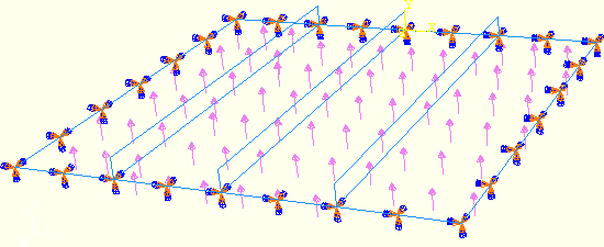
The plate load and boundary conditions are shown in Figure 10–32.
Creating the mesh and defining a job
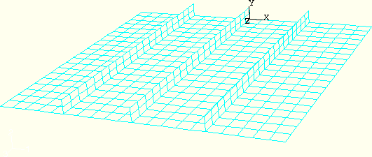
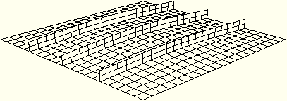
Seed the part with a global element size of 0.1. In addition, select Seed![]() Edge By Number and specify that two elements be created along the height of the stiffeners. Mesh the plate and stiffeners using quadrilateral shell elements (S4R) from the Explicit element library. The resulting mesh is shown in Figure 10–33. This relatively coarse mesh provides moderate accuracy while keeping the solution time to a minimum.
Edge By Number and specify that two elements be created along the height of the stiffeners. Mesh the plate and stiffeners using quadrilateral shell elements (S4R) from the Explicit element library. The resulting mesh is shown in Figure 10–33. This relatively coarse mesh provides moderate accuracy while keeping the solution time to a minimum.
Create a job named BlastLoad. Specify the following job description: Blast load on a flat plate with stiffeners: S4R elements (20x20 mesh) Normal stiffeners (20x2).
Save your model in a model database file, and submit the job for analysis. Monitor the solution progress; correct any modeling errors that are detected, and investigate the cause of any warning messages.
When the job completes, enter the Visualization module, and open the .odb file created by this job (BlastLoad.odb). By default, ABAQUS plots the undeformed model shape with the shaded render style.
Changing the view
The default view is isometric, which does not provide a particularly clear view of the plate. To improve the viewpoint, rotate the view using the options in the View menu or the view tools in the toolbar. Select the viewpoint method for rotating the view. Enter the X-, Y-, and Z-coordinates of the viewpoint vector as 1,0.5,1 and the coordinates of the up vector as 0,1,0.
Animation of results
As noted in earlier examples, animating your results will provide a general understanding of the dynamic response of the plate under the blast loading. First, plot the deformed model shape. Then, create a time-history animation of the deformed shape. Use the Animation Options dialog box to change the mode to Play once.
You will see from the animation that as the blast loading is applied, the plate begins to deflect. Over the duration of the load the plate begins to vibrate and continues to vibrate after the blast load has dropped to zero. The maximum displacement occurs at approximately 8 ms, and a displaced plot of that state is shown in Figure 10–34.
The animation images can be saved to a file for playback at a later time.To save the animation:
From the main menu bar, select Animate![]() Save As.
Save As.
The Save Image Animation dialog box appears.
In the Settings field, enter the file name blast_base.
The format of the animation can be specified as AVI, QuickTime, VRML, or Compressed VRML.
Choose the QuickTime format, and click OK.
The animation is saved as blast_base.mov in your current directory. Once saved, your animation can be played external to ABAQUS/CAE using industry-standard animation software.
History output
Since it is not easy to see the deformation of the plate from the deformed plot, it is desirable to view the deflection response of the central node in the form of a graph. The displacement of the node in the center of the plate is of particular interest since the largest deflection occurs at this node.
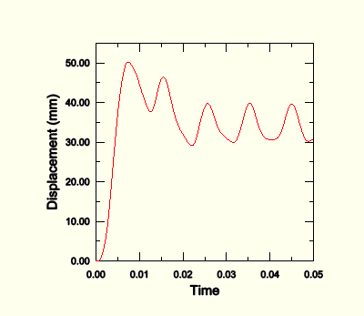
Display the displacement history of the central node, as shown in Figure 10–35 (with displacements in millimeters).
To generate a history plot of the central node displacement:
In the Results Tree, double-click the history output data named Spatial displacement: U2 at the node in the center of the plate (set Center).
Save the current X–Y data: in the Results Tree, click mouse button 3 on the data name and select Save As from the menu that appears. Name the data DISP.
The units of the displacements in this plot are meters. Modify the data to create a plot of displacement (in millimeters) versus time by creating a new data object.
In the Results Tree, expand the XYData container.
The DISP data are listed underneath.
In the Results Tree, double-click XYData; then select Operate on XY data in the Create XY Data dialog box. Click Continue.
In the Operate on XY Data dialog box, multiply DISP by 1000 to create the plot with the displacement values in millimeters instead of meters. The expression at the top of the dialog box should appear as:
"DISP" * 1000
Click Plot Expression to see the modified X–Y data. Save the data as U_BASE2.
Close the Operate on XY Data dialog box.
In the Results Tree, expand the XYPlots container. Click mouse button 3 on XYPlot-1, and select XY Plot Options from the menu that appears. In the XY Plot Options dialog box, change the Y-axis title to Displacement (mm). Click OK to close the dialog box. The resulting plot is shown in Figure 10–35.
The plot shows that the displacement reaches a maximum of 52.1 mm at 7.7 ms and then oscillates after the blast load is removed.
To generate history plots of the model energies:
Save the history results for the ALLKE, ALLSE, ALLPD, ALLIE, and ALLAE output variables as X–Y data.
In the Results Tree, expand the XYData container.
The ALLAE, ALLKE, ALLSE, ALLPD, and ALLIE X–Y data objects are listed underneath.
Select ALLAE, ALLKE, ALLSE, ALLPD, and ALLIE using [Ctrl]+Click; click mouse button 3, and select Plot from the menu that appears to plot the energy curves.
To more clearly distinguish between the different curves in the plot, open the XY Curve Options dialog box and change their line styles.
For the curve ALLSE, select a dashed line style.
For the curve ALLPD, select a dotted line style.
For the curve ALLAE, select a chain dashed line style.
For the curve ALLIE, select the second thinnest line type.
Customize the appearance of the plot further using the XY Plot Options dialog box. Change the title for the Y-axis to Energy.
To change the position of the legend, select Viewport![]() Viewport Annotation Options.
Viewport Annotation Options.
Click the Legend tab.
The position of the upper left corner of the legend is determined by the values specified for % Viewport X and % Viewport Y.
Change the % Viewport X value to 55, and the % Viewport Y value to 50.
This will position the legend so that the upper left corner is 55% of the way across the viewport from left to right and 50% of the way up the viewport from bottom to top.
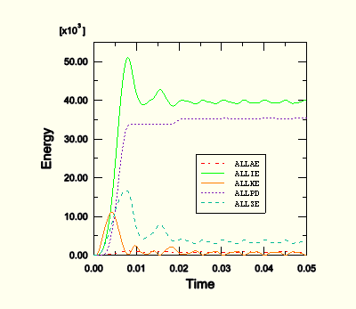
Click OK. The resulting plot is shown in Figure 10–36.
We can see that once the load has been removed and the plate vibrates freely, the kinetic energy increases as the strain energy decreases. When the plate is at its maximum deflection and, therefore, has its maximum strain energy, it is almost entirely at rest, causing the kinetic energy to be at a minimum.
Note that the plastic strain energy rises to a plateau and then rises again. From the plot of kinetic energy we can see that the second rise in plastic strain energy occurs when the plate has rebounded from its maximum displacement and is moving back in the opposite direction. We are, therefore, seeing plastic deformation on the rebound after the blast pulse.
Even though there is no indication that hourglassing is a problem in this analysis, study the artificial strain energy to make sure. As discussed in Chapter 4, “Using Continuum Elements,” artificial strain energy or “hourglass stiffness” is the energy used to control hourglass deformation, and the output variable ALLAE is the accumulated artificial strain energy. This discussion on hourglass control applies equally to shell elements. Since energy is dissipated as plastic deformation as the plate deforms, the total internal energy is much greater than the elastic strain energy alone. Therefore, it is most meaningful in this analysis to compare the artificial strain energy to an energy quantity that includes the dissipated energy as well as the elastic strain energy. Such a variable is the total internal energy, ALLIE, which is a summation of all internal energy quantities. The artificial strain energy is approximately 2% of the total internal energy, indicating that hourglassing is not a problem.
One thing we can notice from the deformed shape is that the central stiffener is subject to almost pure in-plane bending. Using only two first-order, reduced-integration elements through the depth of the stiffener is not sufficient to model in-plane bending behavior. While the solution from this coarse mesh appears to be adequate since there is little hourglassing, for completeness we will study how the solution changes when we refine the mesh of the stiffener. Remember that caution must be taken when refining the mesh, since mesh refinement will increase the solution time by increasing the number of elements and decreasing the element size.
Edit the mesh, and respecify the mesh density. Specify four elements through the height of each stiffener, and remesh the part instance. Create a new job named BlastLoadRefined. Submit this job for analysis, and investigate the results when the job has completed running.
This increase in the number of elements increases the solution time by approximately 20%. In addition, the stable time increment decreases by approximately a factor of two as a result of the reduction of the smallest element dimension in the stiffeners. Since the total increase in solution time is a combination of the two effects, the solution time of the refined mesh increases by approximately a factor of 1.2 × 2, or 2.4, over that of the original mesh.
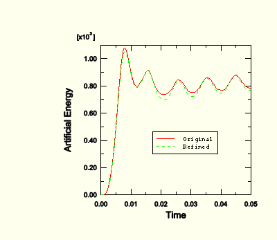
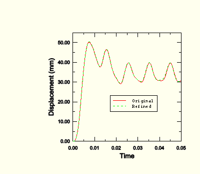
Figure 10–37 shows the histories of artificial energy for both the original mesh and the mesh with the refined stiffeners. The artificial energy is slightly lower in the refined mesh. As a result, we would not expect the results to change significantly from the original to the refined mesh.
Figure 10–38 shows that the displacement of the plate's central node is almost identical in both cases, indicating that the original mesh is capturing the overall response adequately. One advantage of the refined mesh, however, is that it better captures the variation of stress and plastic strain through the stiffeners.Contour plots
In this section you will use the contour plotting capability of the Visualization module to display the von Mises stress and equivalent plastic strain distributions in the plate. Use the model with the refined stiffener mesh to create the plots; from the main menu bar, select File![]() Open and choose the file BlastLoadRefined.odb.
Open and choose the file BlastLoadRefined.odb.
To generate contour plots of the von Mises stress and equivalent plastic strain:
From the main menu bar, select Result![]() Field Output.
Field Output.
In the Field Output dialog box that appears, select the stress output variable (S) from the Output Variable area. The stress invariants are displayed in the Invariant area. Select the Mises stress invariant.
Click Section Points to select a section point.
In the Section Points dialog box that appears, select Top and bottom as the active locations and click OK.
In the Select Plot State dialog box that appears, toggle on Contour and click OK.
ABAQUS plots the contours of the von Mises stress on both the top and bottom faces of each shell element. To see this more clearly, rotate the model in the viewport.
The view that you set earlier for the animation exercise should be changed so that the stress distribution is clearer. You will also need to reposition the legend in the plot.
From the main menu bar, select View![]() Views Toolbox. In the Views dialog box that appears, select the isometric view.
Views Toolbox. In the Views dialog box that appears, select the isometric view.
To change the legend position back to the default position, select Viewport![]() Viewport Annotation Options from the main menu bar. Under the Legend tab in the Viewport Annotation Options dialog box, click Defaults to reset the legend position to its default location.
Viewport Annotation Options from the main menu bar. Under the Legend tab in the Viewport Annotation Options dialog box, click Defaults to reset the legend position to its default location.
Click OK.
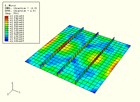
Figure 10–39 shows a contour plot of the von Mises stress at the end of the analysis.
Similarly, contour the equivalent plastic strain. From the main menu bar, select Result![]() Field Output. Select the equivalent plastic strain output variable (PEEQ) from the list of primary output variables, and click OK.
Field Output. Select the equivalent plastic strain output variable (PEEQ) from the list of primary output variables, and click OK.
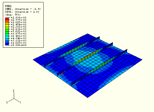
Figure 10–40 shows a contour plot of the equivalent plastic strain at the end of the analysis.
The objective of this analysis is to study the deformation of the plate and the stress in various parts of the structure when it is subjected to a blast load. To judge the accuracy of the analysis, you will need to consider the assumptions and approximations made and identify some of the limitations of the model.
Damping
Undamped structures continue to vibrate with constant amplitude. Over the 50 ms of this simulation, the frequency of the oscillation can be seen to be approximately 214 Hz. A constant amplitude vibration is not the response that would be expected in practice since the vibrations in this type of structure would tend to die out over time and effectively disappear after 5–10 oscillations. The energy loss typically occurs by a variety of mechanisms including frictional effects at the supports and damping by the air.
Consequently, we need to consider the presence of damping in the analysis to model this energy loss. The energy dissipated by viscous effects, ALLVD, is nonzero in the analysis, indicating that there is already some damping present. By default, a bulk viscosity damping (discussed in Chapter 9, “Nonlinear Explicit Dynamics”) is always present and is introduced to improve the modeling of high-speed events.
In this shell model only linear damping is present. With the default value the oscillations would eventually die away, but it would take a long time because the bulk viscosity damping is very small. Material damping should be used to introduce a more realistic structural response. Thus, modify the material definition.
To add damping to a material:
In the Model Tree, double-click Steel underneath the Materials container.
In the Edit Material dialog box, select Mechanical![]() Damping and specify 50 as the value for the mass proportional damping factor, Alpha. Beta is the parameter that controls stiffness proportional damping; at this stage, leave it set to zero.
Damping and specify 50 as the value for the mass proportional damping factor, Alpha. Beta is the parameter that controls stiffness proportional damping; at this stage, leave it set to zero.
Click OK.
The time period for the oscillation of the plate is approximately 10 ms, so we need to increase the analysis period to allow enough time for the vibration to be damped out. Edit the step definition, and increase the time period of step Blast to 150E-3 s.
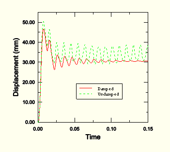
The results of the damped analysis clearly show the effect of mass proportional damping. Figure 10–41 shows the displacement history of the central node for both the damped and undamped analyses. (We have extended the analysis time to 150 ms for the undamped model to compare the data more effectively.) The peak response is also reduced due to damping. By the end of the damped analysis the oscillation has decayed to a nearly static condition.
Rate dependence
Some materials, such as mild steel, show an increase in the yield stress with increasing strain rate. In this example the loading rate is high, so strain-rate dependence is likely to be important.
Add rate dependence to your material definition.
To add rate dependence to your metal plasticity material model:
In the Model Tree, double-click Steel underneath the Materials container.
In the Edit Material dialog box, select Mechanical![]() Plasticity
Plasticity![]() Plastic.
Plastic.
Select Suboptions![]() Rate Dependent.
Rate Dependent.
In the Suboption Editor that appears, enter a value of 40.0 for the Multiplier and a value of 5.0 for the Exponent, and click OK.
Change the time period of step Blast back to the original value of 50 ms. Create a job named BlastLoadRateDep, and submit the job for analysis. When the analysis is complete, open the output database file BlastLoadRateDep.odb, and postprocess the results.
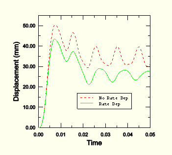
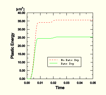
When rate dependence is included, the yield stress effectively increases as the strain rate increases. Therefore, because the elastic modulus is higher than the plastic modulus, we expect a stiffer response in the analysis with rate dependence. Both the displacement history of the central portion of the plate shown in Figure 10–42 and the history of plastic strain energy shown in Figure 10–43 confirm that the response is indeed stiffer when rate dependence is included. The results are, of course, sensitive to the material data. In this case the values of ![]() and
and ![]() are typical of a mild steel, but more precise data would be required for detailed design analyses.
are typical of a mild steel, but more precise data would be required for detailed design analyses.