You have been asked to investigate what happens if the steel connecting lug from Chapter 4, “Using Continuum Elements,” is subjected to an extreme load (60 kN) caused by an accident. The results from the linear analysis indicate that the lug will yield. You need to determine the extent of the plastic deformation in the lug and the magnitude of the plastic strains so that you can assess whether or not the lug will fail. You do not need to consider inertial effects in this analysis; thus, you will use ABAQUS/Standard to examine the static response of the lug.
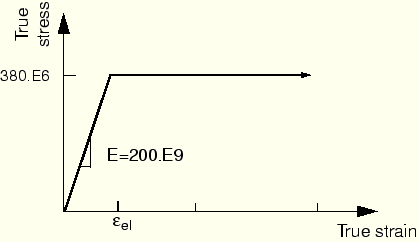
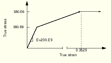
The only inelastic material data available for the steel are its yield stress (380 MPa) and its strain at failure (0.15). You decide to assume that the steel is perfectly plastic: the material does not harden, and the stress can never exceed 380 MPa (see Figure 10–8).
In reality some hardening will probably occur, but this assumption is conservative; if the material hardens, the plastic strains will be less than those predicted by the simulation.A Python script is provided in “Connecting lug with plasticity,” Section A.8. When this script is run through ABAQUS/CAE, it creates the complete analysis model for this problem. Run this script if you encounter difficulties following the instructions given below or if you wish to check your work. Instructions on how to run the script are given in Appendix A, “Example Files.”
If you do not have access to ABAQUS/CAE or another preprocessor, the input file required for this problem can be created manually, as discussed in “Example: connecting lug with plasticity,” Section 8.4 of Getting Started with ABAQUS/Standard: Keywords Version.
Open the model database file Lug.cae, and copy the model Elastic to a model named Plastic.
Material definition
For the Plastic model, you will specify the post-yield behavior of the material using the classical metal plasticity model in ABAQUS. The initial yield stress at zero plastic strain is 380 MPa. Since you are modeling the steel as perfectly plastic, no other yield stresses are required. You will perform a general, nonlinear simulation because of the nonlinear material behavior in the model.
To add plasticity data to the material model:
In the Model Tree, expand the Materials container and double-click Steel.
In the material editor, select Mechanical![]() Plasticity
Plasticity![]() Plastic to invoke the classical metal plasticity model. Enter an initial yield stress of 380.E6 with a corresponding initial plastic strain of 0.0.
Plastic to invoke the classical metal plasticity model. Enter an initial yield stress of 380.E6 with a corresponding initial plastic strain of 0.0.
Step definition and output requests
Edit the step definition and output requests. In the Basic tabbed page of the Edit Step dialog box, set the total time period to 1.0. Assume that the effects of geometric nonlinearity will not be important in this simulation. In the Incrementation tabbed page, specify an initial increment size that is 20% of the total step time (0.2). This simulation is a static analysis of the lug under extreme loads; you do not know in advance how many increments this simulation may require. The default maximum of 100 increments, however, is reasonably large and should be sufficient for this analysis.
Open the Field Output Requests Manager. Edit the current output request to request the default preselected field data at every increment.
Loading
The load applied in this simulation is twice what was applied in the linear elastic simulation of the lug (60 kN vs. 30 kN). Therefore, in the Model Tree, double-click Pressure load underneath the Loads container, and double the magnitude of the pressure applied to the lug (i.e., change the magnitude to 10.0E7).
Job definition
In the Model Tree, create a job named PlasticLugNoHard, and enter the following job description: Elastic-Plastic Steel Connecting Lug. Remember to save your model database file.
Submit the job for analysis, and monitor the solution progress. Correct any modeling errors, and investigate the source of any warning messages. This analysis should terminate prematurely; the reasons are discussed in the following section.
You can monitor the progress of your analysis while it is running by looking at the Job Monitor.
Job Monitor
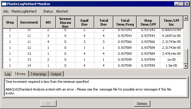
When ABAQUS/Standard has finished the simulation, the Job Monitor will contain information similar to that shown in Figure 10–9.
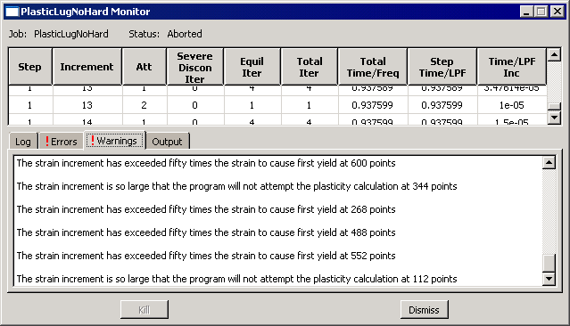
ABAQUS/Standard was able to apply only 94% of the prescribed load to the model and still obtain a converged solution. The Job Monitor shows that ABAQUS/Standard reduced the size of the time increment, shown in the last (right-hand) column, many times during the simulation and stopped the analysis in the fourteenth increment. The information on the Errors tabbed page (see Figure 10–9) indicates that the analysis terminated because the size of the time increment is smaller than the value allowed for this analysis. This is a classic symptom of convergence difficulties and is a direct result of the continued reduction in the time increment size. To begin diagnosing the problem, click the Warnings tab in the Job Monitor dialog box. As shown in Figure 10–10, many warning messages concerning large strain increments and problems with the plasticity calculations are found here. These warnings are related since problems with the plasticity calculations are typically the result of excessively large strain increments and often lead to divergence. Thus, we suspect that numerical problems with the plasticity calculations caused ABAQUS/Standard to terminate the analysis early.Job diagnostics
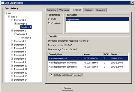
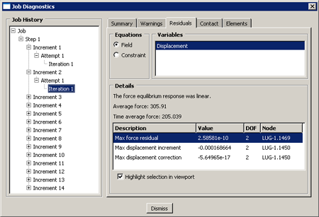
Enter the Visualization module, and open the file PlasticLugNoHard.odb. Open the Job Diagnostics dialog box to examine the convergence history of the job. Looking at the information for the first increment in the analysis (see Figure 10–11), you will discover that the model's initial behavior is assumed to be linear. This judgement is based on the fact that the magnitude of the residual, ![]() , is less than 10–8
, is less than 10–8![]() (the time average force); the displacement correction criterion is ignored in this case.
(the time average force); the displacement correction criterion is ignored in this case.
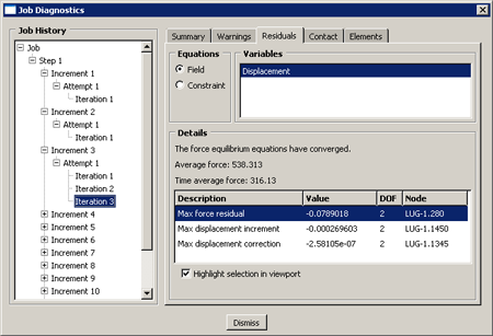
ABAQUS/Standard requires several iterations to obtain a converged solution in the third increment, which indicates that nonlinear behavior occurs in the model during this increment. The only nonlinearity in the model is the plastic material behavior, so the steel must have started to yield somewhere in the lug at this applied load magnitude. The summary of the final (converged) iteration for the third increment is shown in Figure 10–13.
ABAQUS/Standard attempts to find a solution in the fourth increment using an increment size of 0.3, which means it is applying 30% of the total load, or 18 kN, during this increment. After several iterations, ABAQUS/Standard abandons the attempt and reduces the size of the time increment to 25% of the value used in the first attempt. This reduction in increment size is called a cutback. With the smaller increment size, ABAQUS/Standard finds a converged solution in just a few iterations.
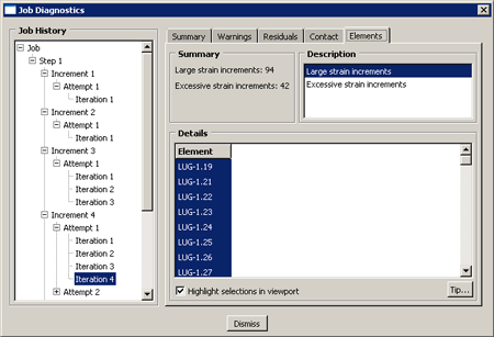
Look more closely at the information for the first attempt of the fourth increment (this is where the convergence difficulties first appear). For this attempt ABAQUS/Standard detects large strain increments at the integration points of a number of elements, as shown in Figure 10–14. “Large” strain increments are those that exceed the strain at initial yield by 50 times; some of these increments are also considered “excessive,” which implies the plasticity calculations are not even attempted at the affected integration points. Thus, we see that the onset of the convergence difficulties is directly related to the large strain increments and problems with the plasticity calculations.
ABAQUS/Standard encounters renewed convergence difficulties in subsequent increments until finally it terminates the job. In many of these increments ABAQUS/Standard cuts back the time increment size because the strain increments are so large that the plasticity calculations are not even performed. Thus, we conclude the overall convergence difficulties are indeed the result of numerical problems with the plasticity calculations.
This check on the magnitude of the total strain increment is an example of the many automatic solution controls ABAQUS/Standard uses to ensure that the solution obtained for your simulation is both accurate and efficient. The automatic solution controls are suitable for almost all simulations. Therefore, you do not have to worry about providing parameters to control the solution algorithm: you only have to be concerned with the input data for your model.
An interesting observation is made using the Job Diagnostics dialog box: in virtually all attempts where convergence problems are encountered, the elements with large or excessive strain increments are in the vicinity of the built-in end of the lug (where yielding begins) while the node with the largest displacement correction is in the vicinity of the loaded end of the lug. This implies that the loaded end wants to deform more than the built-in end can support. Deformed model shape plots can help you pursue this observation further.
Look at the results in the Visualization module to understand what caused the excessive plasticity.
Plotting the deformed model shape
Create a plot of the model's deformed shape, and check that this shape is realistic.
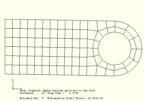
The default view is isometric. You can set the view shown in Figure 10–15 by using the options in the View menu or the view tools in the toolbar; in this figure perspective is also turned off.
The displacements and, particularly, the rotations of the lug shown in the plot are large. Yet they do not seem large enough to have caused all of the numerical problems seen in the simulation. Look closely at the information in the plot's title for an explanation. The deformation scale factor used in this plot is 0.02; i.e., the displacements are scaled to 2% of their actual values. (Your deformation scale factor may be different.)ABAQUS/CAE always scales the displacements in a geometrically linear simulation such that the deformed shape of the model fits into the viewport. (This is in contrast to a geometrically nonlinear simulation, where ABAQUS/CAE does not scale the displacements and, instead, adjusts the view by zooming in or out to fit the deformed shape in the plot.) To plot the actual displacements, set the deformation scale factor to 1.0. This will produce a plot of the model in which the lug has deformed until it is almost parallel to the vertical (global Y) axis.
The applied load of 60 kN exceeds the limit load of the lug, and the lug collapses when the material yields at all the integration points through its thickness. The lug then has no stiffness to resist further deformation because of the perfectly plastic post-yield behavior of the steel. This is consistent with the pattern observed earlier concerning the locations of the large strain increments and maximum displacement corrections.
The connecting lug simulation with perfectly plastic material behavior predicts that the lug will suffer catastrophic failure caused by the collapse of the structure. We have already mentioned that the steel would probably exhibit some hardening after it has yielded. You suspect that including hardening behavior would allow the lug to withstand this 60 kN load because of the additional stiffness it would provide. Therefore, you decide to add some hardening to the steel's material property definition. Assume that the yield stress increases to 580 MPa at a plastic strain of 0.35, which represents typical hardening for this class of steel. The stress-strain curve for the modified material model is shown in Figure 10–16.
Modify your plastic material data so that it includes the hardening data. Edit the material definition to add a second row of data to the plastic data form. Enter a yield stress of 580.E6 with a corresponding plastic strain of 0.35.Create a job named PlasticLugHard. Submit the job for analysis, and monitor the solution progress. Correct any modeling errors, and investigate the source of any warning messages.
Job Monitor
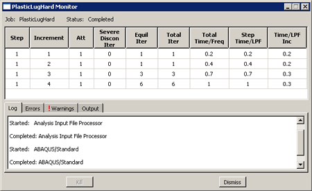
The summary of the analysis in the Job Monitor, shown in Figure 10–17, indicates that ABAQUS/Standard found a converged solution when the full 60 kN load was applied. The hardening data added enough stiffness to the lug to prevent it from collapsing under the 60 kN load.
There are no convergence-related warnings issued during the analysis, so you can proceed directly to postprocessing the results.
Enter the Visualization module, and open the file PlasticLugHard.odb.
Deformed model shape and peak displacements
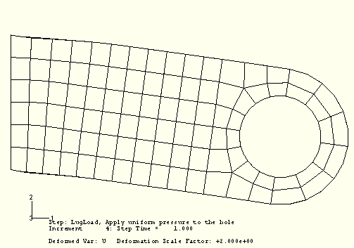
Plot the deformed model shape with these new results, and change the deformation scale factor to 2 to obtain a plot similar to Figure 10–18. The displayed deformations are double the actual deformations.
Contour plot of Mises stress
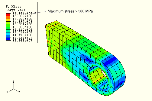
Contour the Mises stress in the model. Create a filled contour plot using ten contour intervals on the actual deformed shape of the lug (i.e., set the deformation scale factor to 1.0) with the plot title and state blocks suppressed. Use the view manipulation tools to position and size the model to obtain a plot similar to that shown in Figure 10–19.
Do the values listed in the contour legend surprise you? The maximum stress is greater than 580 MPa, which should not be possible since the material was assumed to be perfectly plastic at this stress magnitude. This misleading result occurs because of the algorithm that ABAQUS/CAE uses to create contour plots for element variables, such as stress. The contouring algorithm requires data at the nodes; however, ABAQUS/Standard calculates element variables at the integration points. ABAQUS/CAE calculates nodal values of element variables by extrapolating the data from the integration points to the nodes. The extrapolation order depends on the element type; for second-order, reduced-integration elements ABAQUS/CAE uses linear extrapolation to calculate the nodal values of element variables. To display a contour plot of Mises stress, ABAQUS/CAE extrapolates the stress components from the integration points to the nodal locations within each element and calculates the Mises stress. If the differences in Mises stress values fall within the specified averaging threshold, nodal averaged Mises stresses are calculated from each surrounding element's invariant stress value. Invariant values exceeding the elastic limit can be produced by the extrapolation process.
Try plotting contours of each component of the stress tensor (variables S11, S22, S33, S12, S23, and S13). You will see that there are significant variations in these stresses across the elements at the built-in end. This causes the extrapolated nodal stresses to be higher than the values at the integration points. The Mises stress calculated from these values will, therefore, also be higher.
The Mises stress at an integration point can never exceed the current yield stress of the element's material; however, the extrapolated nodal values reported in a contour plot may do so. In addition, the individual stress components may have magnitudes that exceed the value of the current yield stress; only the Mises stress is required to have a magnitude less than or equal to the value of the current yield stress.
You can use the query tools in the Visualization module to check the Mises stress at the integration points.
To query the Mises stress:
From the main menu bar, select Tools![]() Query; or use the
Query; or use the ![]() tool in the toolbar.
tool in the toolbar.
The Query dialog box appears.
In the Visualization Module Queries field, select Probe values.
Click OK.
The Probe Values dialog box appears.
Select the Mises stress output by clicking in the column to the left of S, Mises.
A check mark appears in the S, Mises row.
Make sure that Elements and the output position Integration Pt are selected.
Use the cursor to select elements near the constrained end of the lug.
ABAQUS/CAE reports the element ID and type by default and the value of the Mises stress at each integration point starting with the first integration point. The Mises stress values at the integration points are all lower than the values reported in the contour legend and also below the yield stress of 580 MPa. You can click mouse button 1 to store probed values.
Click Cancel when you have finished probing the results.
The fact that the extrapolated values are so different from the integration point values indicates that there is a rapid variation of stress across the elements and that the mesh is too coarse for accurate stress calculations. This extrapolation error will be less significant if the mesh is refined but will always be present to some extent. Therefore, always use nodal values of element variables with caution.
Contour plot of equivalent plastic strain
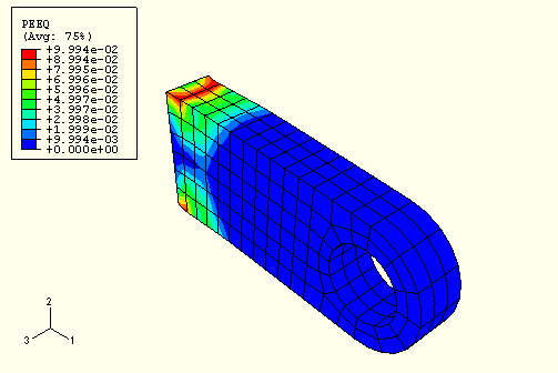
The equivalent plastic strain in a material (PEEQ) is a scalar variable that is used to represent the material's inelastic deformation. If this variable is greater than zero, the material has yielded. Those parts of the lug that have yielded can be identified in a contour plot of PEEQ by selecting Result![]() Field Output from the main menu bar and selecting PEEQ from the list of output variables in the dialog box that appears. Set the colors for values outside the contour limits to Use spectrum min/max (open the Contour Plot Options dialog box and select the Color & Style tab; then select the Spectrum tab). Thus, any areas in the model plotted in dark blue in ABAQUS/CAE still have elastic material behavior (see Figure 10–20).
Field Output from the main menu bar and selecting PEEQ from the list of output variables in the dialog box that appears. Set the colors for values outside the contour limits to Use spectrum min/max (open the Contour Plot Options dialog box and select the Color & Style tab; then select the Spectrum tab). Thus, any areas in the model plotted in dark blue in ABAQUS/CAE still have elastic material behavior (see Figure 10–20).
Creating a variable-variable (stress-strain) plot
The X–Y plotting capability in ABAQUS/CAE was introduced earlier in this manual. In this section you will learn how to create X–Y plots showing the variation of one variable as a function of another. You will use the stress and strain data saved to the output database (.odb) file (in the form of field output rather than history output) to create a stress-strain plot for one of the integration points in an element adjacent to the constrained end of the lug.
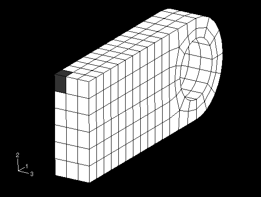
Consider the shaded element shown in Figure 10–21.
Because the stress and strain magnitudes will be largest in this element, you should plot the stress and strain histories at an integration point in this element; the integration point should be chosen so that it is the closest one to the top surface of the lug but not adjacent to the constrained nodes. The numbering of the integration points depends on the element's nodal connectivity. Thus, you will need to identify the element's label as well as its nodal connectivity to determine which integration point to use.To determine the integration point number:
In the toolbar, select the Replace Selected ![]() tool and click the shaded element shown in Figure 10–21.
tool and click the shaded element shown in Figure 10–21.
Plot the undeformed shape of this element with the node labels made visible. Click the auto-fit tool ![]() to obtain a plot similar to Figure 10–22.
to obtain a plot similar to Figure 10–22.
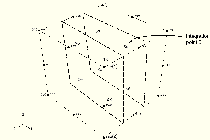
Use the Query tool to obtain the nodal connectivity for this corner element (click in the column to the left of Nodes in the Probe Values dialog box). You will have to expand the Nodes column at the bottom of the dialog box to see the complete list; you are interested in only the first four nodes.
Compare the nodal connectivity list with the undeformed model shape plot to determine which is the 1–2–3–4 face on your C3D20R element, as defined in “Three-dimensional solid element library,” Section 22.1.4 of the ABAQUS Analysis User's Manual. For example, in Figure 10–22 the 276–552–313–79 face corresponds to the 1–2–3–4 face. Thus, the integration points are numbered as shown in the figure. We are interested in the point that corresponds to integration point 5.
In the following discussion, assume that the element label is 41 and that integration point 5 of this element satisfies the requirements stated above. Your element and/or integration point numbers may differ.
To create history curves of stress and direct strain along the lug:
In the Results Tree, double-click XYData.
The Create XY Data dialog box appears.
In this dialog box, select ODB field output as the source and click Continue.
The XY Data from ODB Field Output dialog box appears; the Variables tabbed page is open by default.
In this dialog box, expand the following lists: S: Stress components and E: Strain components.
From the list of available stress and strain components, select Mises and E11, respectively.
The Mises stress, rather than the component of the true stress tensor, is used because the plasticity model defines plastic yield in terms of Mises stress. The E11 strain component is used because it is the largest component of the total strain tensor at this point; using it clearly shows the elastic, as well as the plastic, behavior of the material at this integration point.
Click the Elements/Nodes tab.
Accept Pick from viewport as the selection method, and click Edit Selection.
In the viewport, click on the shaded element shown in Figure 10–21; then click Done in the prompt area.
Click Save to save the data followed by Dismiss to close the dialog box.
Sixteen curves are created (one for each variable at each integration point), and default names are given to the curves. The curves appear in the XYData container. Each of the curves is a history (variable versus time) plot. You must combine the plots for the integration point of interest, eliminating the time dependence, to produce the desired stress-strain plot.
To combine history curves to produce a stress-strain plot:
In the Results Tree, double-click XYData.
The Create XY Data dialog box appears.
Select Operate on XY data, and click Continue.
The Operate on XY Data dialog box appears. Expand the Name field to see the full name of each curve.
From the Operators listed, select combine(X,X).
combine( ) appears in the text field at the top of the dialog box.
In the XY Data field, select the stress and strain curves for the integration point of interest.
Click Add to Expression. The expression combine("E:E11 ...", "S:MISES ...") appears in the text field. In this expression "E:E11 ..." will determine the X-values and "S:MISES ..." will determine the Y-values in the combined plot.
Save the combined data object by clicking Save As at the bottom of the dialog box.
The Save XY Data As dialog box appears. In the Name text field, type SVE11; and click OK to close the dialog box.
To view the combined stress-strain plot, click Plot Expression at the bottom of the dialog box.
Click Cancel to close the dialog box.
This X–Y plot would be clearer if the limits on the X- and Y-axes were changed. Use the XY Plot Options to do this.
To customize the stress-strain curve:
In the Results Tree, expand the XYPlots container. Click mouse button 3 on XYPlot-1, and select XY Plot Options from the menu that appears.
The XY Plot Options dialog box appears.
Set the maximum range of the X-axis (E11 strain) to 0.09, the maximum range of the Y-axis (MISES stress) to 500 MPa, and the minimum stress to 0.0 MPa.
Click the Titles tab, and select User-specified as the Title source for the X- and Y-axes.
Customize the axis labels as they appear in Figure 10–23 by filling in the Title text fields for the X- and Y-axes.
Click OK to close the XY Plot Options dialog box.
It will also be helpful to display a symbol at each data point of the curve. In the Results Tree, expand the XYPlot-1 container. Click mouse button 3 on Curve, and select XY Curve Options from the menu that appears.
The XY Curve Options dialog box appears.
From the XY Data field, select the stress-strain curve (SVE11).
The SVE11 data object is highlighted.
Toggle on Show symbol. Accept the defaults, and click OK at the bottom of the dialog box.
The stress-strain plot appears with a symbol at each data point of the curve.
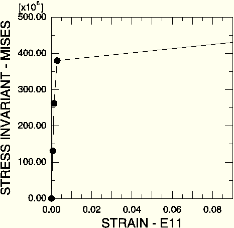
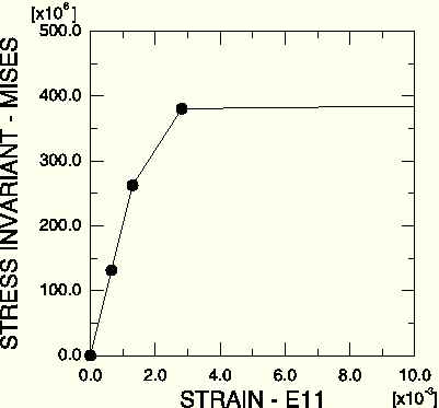
You should now have a plot similar to the one shown in Figure 10–23. The stress-strain curve shows that the material behavior was linear elastic for this integration point during the first two increments of the simulation. In this plot it appears that the material remains linear during the third increment of the analysis; however, it does yield during this increment. This illusion is created by the extent of strain shown in the plot. If you limit the maximum strain displayed to 0.01 and set the minimum value to 0.0, the nonlinear material behavior in the third increment can be seen more clearly (see Figure 10–24).
Figure 10–24 Mises stress vs. direct strain (E11) along the lug in the corner element. Maximum strain 0.01.
The results from this second simulation indicate that the lug will withstand this 60 kN load if the steel hardens after it yields. Taken together, the results of the two simulations demonstrate that it is very important to determine the actual post-yield hardening behavior of the steel. If the steel has very little hardening, the lug may collapse under the 60 kN load. Whereas if it has moderate hardening, the lug will probably withstand the load although there will be extensive plastic yielding in the lug (see Figure 10–20). However, even with plastic hardening, the factor of safety for this loading will probably be very small.