Product: ABAQUS/Standard
This example illustrates the use of the substructure capability in ABAQUS to simulate efficiently the vehicle dynamics of a detailed pick-up truck model going over road bumps. The pick-up truck model geometry described in “Inertia relief in a pick-up truck,” Section 3.2.1, is used in this example. The model is organized as a collection of individual parts that are connected together. Twenty substructures are then created, one for each part that may undergo large motions but for which it is reasonable to assume small-strain elastic deformation (e.g., the chassis). Several parts that may deform nonlinearly (e.g., leaf springs for the rear suspension or the stabilizer bar in the front) are modeled using the usual general nonlinear modeling options. Connection points are created for each part using the *COUPLING option (in most cases). The parts are then attached together using appropriate connector elements. A simplified CALSPAN tire model is used (UEL) to model the radial forces in the tires. The vehicle is loaded statically by gravity, accelerated in a dynamic step on a flat road, and run over bumps. Without stress recovery in the substructures the substructure analysis runs an estimated 120 times faster than an equivalent analysis without substructures.
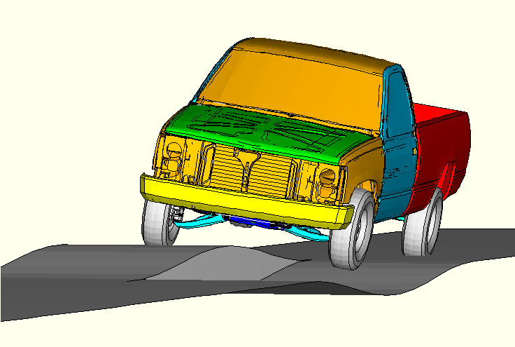
The pick-up truck model (1994 Chevrolet C1500) discussed here is depicted in Figure 3.2.2–1 riding over antisymmetric bumps. The model geometry, element connectivity, and material properties are obtained from the Public Finite Element Model Archive of the National Crash Analysis Center at George Washington University. The materials used are described in “Inertia relief in a pick-up truck,” Section 3.2.1.
The model is organized as a collection of individual parts connected together. Most parts that undergo only small deformations in addition to a large rigid body motion are defined as substructures. Substructures are created for the following parts: the chassis, each of the four A-arms for the front suspension, each of the four wheels, the rear axle, the driveshaft, the engine/transmission, the cabin, each of the two doors, the hood, the seat, the front bumper, the truck bed, and the fuel tank.
The number of retained nodes for each substructure is determined primarily by its connection points with neighboring parts as illustrated in Figure 3.2.2–2 for the cabin substructure. There are twenty points associated with this substructure that are used to connect the cabin to other parts in the model. There are six retained nodes on the cabin bottom (connections to the chassis); three retained nodes for the hood connections (two hinges and the hood lock); three retained nodes for each of the two door connections (two hinges in the front and the door lock in the back); four retained nodes for the seat connections; and one node retained at the center of mass of the vehicle used for yaw, pitch, and roll measurement purposes.
Several parts deform too much to be considered substructures and are modeled using regular elements. The leaf springs in the back and the stabilizer bar in the front are both modeled with beam elements. The front brake assemblies are modeled as rigid bodies.
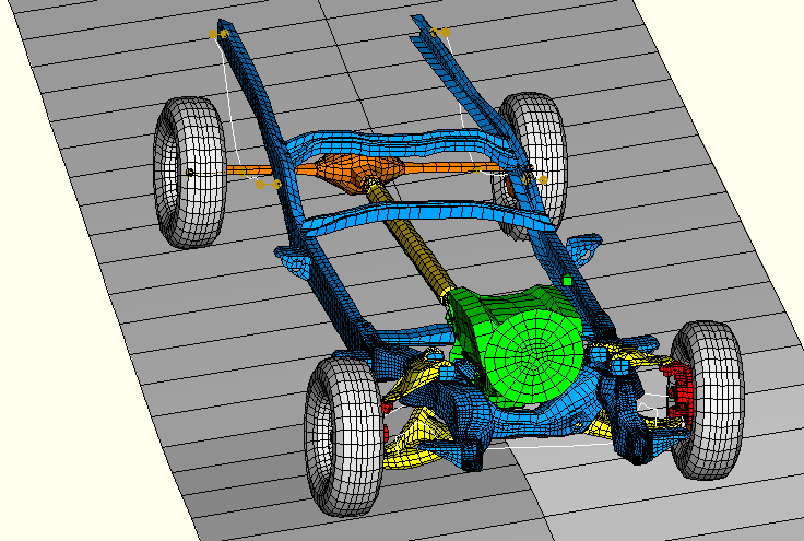
The connections between parts are modeled using connector elements. JOIN and REVOLUTE connectors are used to model the hinges between each of the following parts: the A-arms and chassis, the doors and cabin, the hood and cabin, the wheels and knuckles, and the leaf springs and chassis. CARTESIAN and CARDAN connections with appropriately defined *CONNECTOR ELASTICITY, *CONNECTOR DAMPING, and *CONNECTOR FRICTION options are used to define some of the bushing connections (e.g., engine mounts). Two UNIVERSAL connectors are used to model the driveshaft connections to the transmission in the front and to the differential in the back. BEAM connectors are used to model rigid connections between parts. The *CONNECTOR MOTION option applied to an AXIAL connector is used to lock (or open) the doors and the hood. The *CONNECTOR MOTION option applied to a SLOT connector is used to specify the steering by moving the steering rack. The struts are modeled using an AXIAL connection by specifying approximate nonlinear elasticity and damping. Several of the suspension-related parts are shown in Figure 3.2.2–3.
The radial forces in the tires are modeled approximately using a simplified CALSPAN tire model (Frik, Leister, and Schwartz, 1993) implemented via user subroutine UEL. A radial stiffness of 600 N/mm is considered.
For all analyses the gravity-loaded static equilibrium configuration is found first. Since the given mesh geometry corresponds to the gravity-loaded equilibrium position and data are not available for the pre-stress in the suspension springs and tires, the pre-stress forces have to be computed. To achieve this end, a separate static stress analysis with artificial properties for the suspension springs and artificial boundary conditions is first performed, as follows. The vehicle is supported with boundary conditions in the vertical direction at the four wheel spindles (where the tire UELs will be connected) and fixed at the center of mass to prevent in-plane rigid body motion (degrees of freedom 1, 2, and 6). The stiffnesses of the suspension springs are increased artificially by a thousand times in this independent analysis to minimize deformation. The gravity load is then applied to obtain equilibrium stresses in the suspension components and reaction forces at the wheel spindles.
In the analysis of interest (with realistic properties and boundary conditions), the stresses and reaction forces obtained from the artificial static step are used as initial stresses in the suspension spring components and as pre-stress forces in the tires, respectively. A *STATIC gravity loading step is run to obtain an equilibrium configuration. This equilibrium configuration differs only slightly from the given initial geometry (the wheel spindles move laterally about two millimeters). Thus, the initial stress state in the suspension springs and tires accurately represents static equilibrium, and the vehicle is ready for dynamic loading.
The vehicle model is prescribed an initial velocity and then accelerated (0.5 g) to the desired velocity (5 m/sec or 7 m/sec) in a *DYNAMIC step. Once the “cruise” velocity is achieved, the truck model is run over symmetric or antisymmetric bumps (0.2 m high and 5.0 m long).
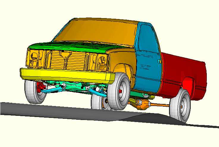
In Figure 3.2.2–4 a snapshot of the truck moving forward with a velocity of 7 m/sec (25.2 km/h) and “jumping” over symmetric bumps is shown. The wheels loose contact with the ground and then land again on the road (not shown).
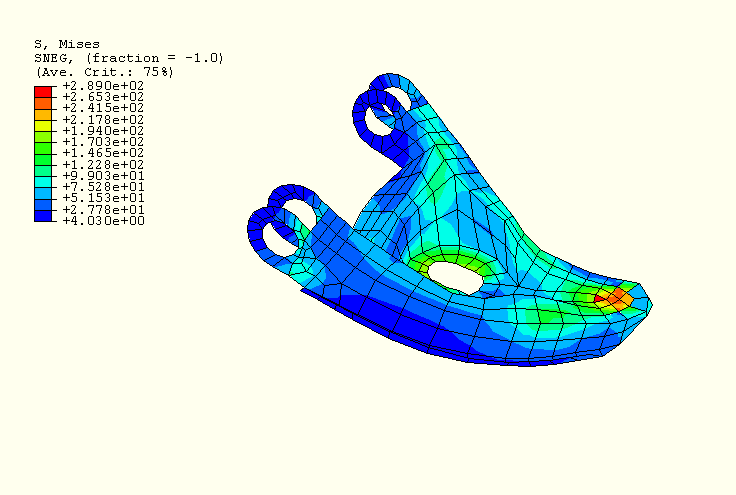
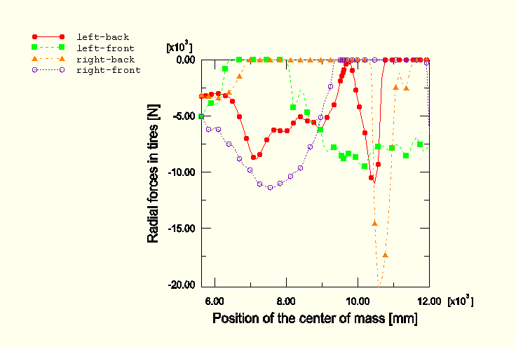
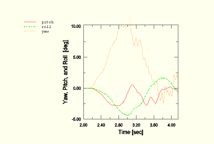
More results are presented for the case when the truck is riding over antisymmetric bumps (see Figure 3.2.2–1). Stresses are recovered for the lower left A-arm substructure and shown in Figure 3.2.2–5 when the front wheels have traveled 3.2 m over the bumps. The radial forces on the tires are shown in Figure 3.2.2–6, beginning from the moment when the front tires are about to go over the bumps. A zero radial force indicates that the tire is out of contact. The yaw, pitch, and roll angles recorded using a CARDAN connector attached to the model at its center of mass are shown in Figure 3.2.2–7.
The advantage of using substructures instead of regular deformable elements becomes obvious when the total times needed to complete these types of analyses are compared. A full analysis using regular elements has not been performed since approximately five CPU days would be necessary to complete either of the two analyses discussed above. This total time was estimated by running a few increments, estimating the time needed per iteration, and then multiplying the time per iteration by the total number of iterations needed to complete the analysis. Using these estimates, the substructure analysis is up to 120 times faster than the regular mesh analysis, depending on the amount of recovery performed for each substructure.
The abaqus substructurecombine execution procedure can combine model and results data from two substructure output databases into a single output database. For more information, see “Execution procedure for combining output from substructures,” Section 3.2.17 of the ABAQUS Analysis User's Manual. To combine the substructure output databases, at least one frame of field output must be requested.
Substructure global analysis of the truck going over in-phase bumps.
Substructure global analysis of the truck going over antiphase bumps.
All node definitions.
*PARAMETER definitions.
All material definitions.
Initial stress definition for the leaf springs.
*CONNECTOR MOTION that keeps the doors and the hood locked.
Output definitions for the substructures.
*RIGID BODY definition of the front left brake assembly.
*RIGID BODY definition of the front right brake assembly.
*PARAMETER definitions for the in-phase analysis.
*PARAMETER definitions for the antiphase analysis.
UEL used to define the tire model.
Chassis.
Retained nodes for the chassis.
Lower left A-arm.
Lower right A-arm.
Upper left A-arm.
Upper right A-arm.
Rear axle.
Retained nodes for the rear axle.
Engine and transmission.
Driveshaft.
Cabin and front fenders.
Retained nodes for the cabin.
Hood.
Left door.
Right door.
Seat.
Truck bed.
Fuel tank.
Front bumper.
Rear left wheel.
Rear right wheel.
Front left wheel.
Front right wheel.
Rear leaf spring suspension.
Front stabilizer bar.
Steering rods and steering rack.
Chassis.
Lower left A-arm.
Lower right A-arm.
Upper left A-arm.
Upper right A-arm.
Rear axle.
Engine and transmission.
Driveshaft.
Cabin and front fenders.
Hood.
Left door.
Right door.
Seat.
Truck bed.
Fuel tank.
Front bumper.
Rear left wheel.
Rear right wheel.
Front left wheel.
Front right wheel.
Chassis.
Engine and transmission.
Cabin and front fenders.
Hood.
Left door.
Right door.
Seat.
Fuel tank.
Front bumper.
Chassis.
Lower left A-arm.
Lower right A-arm.
Upper left A-arm.
Upper right A-arm.
Rear axle.
Engine and transmission.
Driveshaft.
Cabin and front fenders.
Hood.
Left door.
Right door.
Seat.
Truck bed.
Fuel tank.
Front bumper.
Rear left wheel.
Rear right wheel.
Front left wheel.
Front right wheel.
Left A-arms.
Right A-arms.
Left front brake assembly.
Right front brake assembly.
Steering rods.
Stabilizer bar.
Leaf springs.
Engine and transmission.
Driveshaft.
Cabin to chassis.
Hood.
Left door.
Right door.
Seat.
Truck bed.
Fuel tank.
Front bumper.
Rear wheels.
Front wheels.
Frik, S., G. Leister, and W. Schwartz, “Simulation of the IAVSD Road Vehicle Benchmark Bombardier Iltis with FASIM, MEDYNA, NEWEUL, and SIMPACK,” in Multibody Computer Codes in Vehicle System Dynamics, Ed. W. Kortum and R. S. Sharp, February 1993.