Product: ABAQUS/Standard
This example illustrates how to perform inertia relief (“Inertia relief,” Section 11.1.1 of the ABAQUS Analysis User's Manual) in a static analysis in ABAQUS/Standard. The problem involves stopping a pick-up truck, moving with an initial velocity of 50.0 km/h (13.89 m/s), by applying braking loads. Inertia relief is used here to supply inertia forces in a static analysis that oppose the braking loads specified in the model. The solution provides the rigid body deceleration and the static stresses in the pick-up truck. For comparison purposes a dynamic analysis is performed with the same initial velocity and braking loads.
A 1994 Chevrolet C1500 pick-up truck (see Figure 3.2.1–1) is modeled using approximately 55,000 elements. The model was obtained from the Public Finite Element Model Archive of the National Crash Analysis Center at George Washington University. The finite element model was converted into an ABAQUS/Standard input file, and several missing constraints were added to carry out the analyses. The model consists of various parts—such as cabin, truck bed, doors, etc.—which are meshed with shell elements, three-dimensional beam elements, and three-dimensional solid elements. The parts are attached with connector elements, coupling elements, and multi-point constraints.
The materials used in the truck model are idealized as elastic or elastic-plastic. Suitable adjustments are made to the material properties to account for unmodeled features of various parts such as the internal details of the engine, gearbox, etc. A summary of the material properties and the parts for which they are used is given in Table 3.2.1–1 and Table 3.2.1–2.
Rigid body definitions are used for brakes and brake assemblies to take advantage of the high stiffness of these parts relative to other parts. Connector elements are used to model kinematic constraints governing relative motions between various parts (see “Substructure analysis of a pick-up truck model,” Section 3.2.2, for details).
The finite element model of the truck is oriented such that the positive 1-direction goes from the rear to the front of the truck, the positive 2-direction goes from the passenger (right-hand) side to the driver (left-hand) side, and the positive 3-direction is upward. In this system the braking loads are applied at the respective wheel spindles as concentrated forces in the negative 1-direction.
To simplify the analysis, normal contact between the tires and the road surface is modeled through spring elements that have one node connected to the wheel spindle and the other node fixed against displacement in the 3-direction and kinematically constrained to the wheel spindle in the other directions. Friction between the tires and the road surface is assumed to be nonexistent. This allows the truck to translate freely in the 1- and 2-directions and rotate freely about the 3-direction; the constraints on the spring nodes prevent translation in the 3-direction and rotation about the 1- and 2-directions.
A separate static analysis is performed to obtain the correct initial configuration and stress distribution under the applied gravity load. The details of this analysis are explained in “Substructure analysis of a pick-up truck model,” Section 3.2.2. This gives us the base state for the analysis of interest.
The total braking load for the truck moving at 13.89 m/s is computed by assuming the truck to be a rigid body that comes to rest over a distance of 20 m after the brakes are applied. This gives a deceleration of 4.82 m/s2 in the 1-direction for the truck. The total mass of the truck as computed from the finite element analysis is 1.72 × 10³ kg, which gives the total inertial force resisted by the brakes (or braking load) as 8.30 kN. Assuming that the front brakes provide 75% of the total resistance and the rear brakes provide the remaining 25%, the braking load for each of the front wheels is 3.11 kN and the braking load for each of the rear wheels is 1.04 kN. The four braking loads applied to the truck are balanced in a static analysis with an inertia relief load. The inertia relief load represents the dynamic effects (not modeled otherwise in a static analysis) of a constant deceleration from the truck's travel velocity to a complete stop.
Since the truck is free to translate in the 1- and 2-directions and rotate about the 3-direction, inertia relief is performed in these three directions. The other directions are constrained by boundary conditions as explained in the previous section.
For comparison purposes a transient dynamic analysis is also performed (after the initial static equilibrium under gravity load) in which the truck is accelerated from zero velocity to the final uniform velocity of 13.89 m/s. This dynamic analysis step is followed by another dynamic analysis step in which the braking loads are applied to bring the truck to a complete stop. The braking loads are ramped up smoothly from zero to the maximum value over 0.5 seconds and then kept constant for 2.88 seconds—the time required to bring the truck to rest from the initial velocity of 13.89 m/s with an average deceleration of 4.82 m/s2. To minimize the analysis time, substructures are used in the dynamic analysis for all deformable parts except the chassis and suspension components, which are modeled as fully deformable since they are the parts that show significant stresses.
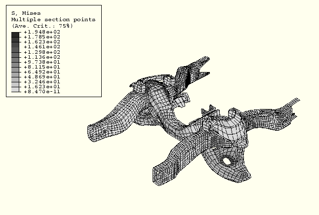
The results for inertia relief in the pick-up truck model with braking loads show that the truck decelerates at 4.83 m/s2 in the 1-direction. The truck has an angular acceleration of 0.01 rad/s2 about the 3-direction at the center of mass due to asymmetry in the distribution of mass. The vertical displacements at the wheel spindles (the front wheel spindles dip about 0.7 mm, and the rear wheel spindles rise about 0.7 mm without loss of contact between tires and the road surface) indicate that the truck pitches forward due to the braking action. A plot of the Mises stress shown in Figure 3.2.1–2 indicates that the largest stresses occur in the suspension components and the regions where the suspension components are connected to the chassis. Plots of the active yield flag and equivalent plastic strains (not shown) indicate that there is no plastic yielding in any part of the truck.
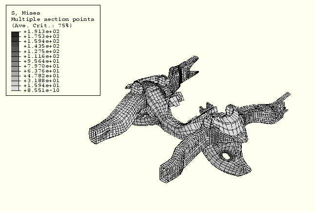
The results for the transient dynamic analysis indicate that the average deceleration after the full braking load has been applied is around 4.94 m/s2 in the 1-direction and the average angular acceleration about the 3-direction is 0.03 rad/s2. The truck pitches forward with the front wheel spindles dipping about 0.7 mm and the rear wheel spindles rising about 0.7 mm in the braking load step. The Mises stress for the dynamic analysis, shown in Figure 3.2.1–3, shows a distribution similar to that obtained for inertia relief. There is no plastic yielding in the chassis or suspension components.
Inertia relief relies on the assumption that the body undergoing loading is free to translate and rotate as a rigid body. Therefore, no external or internal constraints are allowed in the free directions (with the exception of the case where statically determinant boundary conditions are applied and all available directions are considered inertia relief directions). In a complex model like the pick-up truck, with various kinematic constraints and large geometry changes, it is necessary to ensure that the base state for the step including inertia relief is converged to a tight residual tolerance. If it is not converged to a tight tolerance, the out-of-balance forces and moments in the base state will act as internal constraints on rigid body motions. Hence, such unequilibrated forces and moments may prevent a geometrically linear or nonlinear analysis from converging. In this example the *CONTROLS option is used to tighten the convergence tolerance in the gravity load step preceding the inertia relief step.
The comparison of results for inertia relief and dynamic analysis of the truck shows that inertia relief is an inexpensive alternative to dynamic analysis for obtaining the steady-state response of a dynamic system for certain loading situations. In this braking analysis, for example, the static analysis with inertia relief runs about 10 times faster than the general deformable transient dynamic simulation.
Static equilibrium analysis for gravity load and initial stresses followed by inertia relief with braking loads.
Static equilibrium analysis for gravity load and initial stresses followed by dynamic acceleration to uniform velocity and deceleration with braking loads.
The model data are contained in multiple smaller files and referenced as *INCLUDE files in the main input files. The *INCLUDE file names are given in “Substructure analysis of a pick-up truck model,” Section 3.2.2.
Table 3.2.1–1 Properties for elastic-plastic materials used in the truck model.
| Elastic-Plastic Material Name | Properties | Part Name | |||
|---|---|---|---|---|---|
| E (N/m2) | | | |||
| Steel | 2.1 × 10¹¹ | 0.3 | 2.7 × 10⁸ | 7.89 × 10³ | rail (chassis), engine oil box, radiator mounting, fenders, wheel housings, cabin, bed, fan center, fuel tank, rear rim, steering support, battery tray, seat track, radiator outer |
| Steel | 2.1 × 10¹¹ | 0.3 | 3.5 × 10⁸ | 7.89 × 10³ | engine mountings, radiator mountings, radiator, fender mountings, hood, doors, cabin hinges |
| Plastic | 2.8 × 10⁹ | 0.3 | 4.5 × 10⁷ | 1.2 × 10³ | fan cover |
| Glass | 7.6 × 10¹⁰ | 0.3 | 1.38 × 10⁸ | 2.5 × 10³ | windows, windshield |
| Plastic | 3.4 × 10⁹ | 0.3 | 1.0 × 10⁸ | 1.1 × 10³ | radiator side block |
| Plastic | 3.4 × 10⁹ | 0.3 | 1.0 × 10⁸ | 7.1 × 10³ | dashboard interior |
Table 3.2.1–2 Properties for elastic materials used in the truck model.
| Elastic Material Name | Properties | Part Name | ||
|---|---|---|---|---|
| E (N/m2) | | |||
| Steel | 2.1 × 10¹¹ | 0.3 | 7.89 × 10³ | A-arm mountings, fan, door lock beams, headrest connector beams, radiator mounting beams, oil pan beams, rear axle, drive shaft, steering, A-arm-rim connectors, A-arm-rail connectors, bed-rail connector, dashboard support, steering column, rail connector, brakes, gearbox CV joint, front rim |
| Steel | 1.2 × 10¹¹ | 0.3 | 3.89 × 10³ | engine gearbox |
| Steel | 2.1 × 10¹⁰ | 0.3 | 1.82 × 10³ | engine front |
| Steel | 2.1 × 10¹¹ | 0.3 | 2.5 × 10³ | door lock |
| Rubber | 2.461 × 10⁹ | 0.323 | 8.0598 × 10³ | tires |
| Steel | 2.1 × 10¹¹ | 0.3 | 3.5765 × 10³ | rear suspension |
| Steel | 2.1 × 10¹¹ | 0.3 | 2.089 × 10⁴ | brake assembly |
| Steel | 2.1 × 10¹¹ | 0.3 | 6.911 × 10³ | brake assembly |
| Rubber-Metal Composite | 2.1 × 10¹¹ | 0.3 | 1.96 × 10³ | battery |
| Foam | 2.0 × 10⁹ | 0.3 | 2.527 × 10² | seat bottom |
| Foam | 2.0 × 10⁹ | 0.3 | 7.55 × 10² | seat top |
| Foam | 2.0 × 10⁹ | 0.3 | 1.69 × 10² | seat headrest |