Product: ABAQUS/Standard
This example illustrates the use of the *STEADY STATE DYNAMICS, SUBSPACE PROJECTION option to model the frequency response of a tire about a static footprint solution.
The *STEADY STATE DYNAMICS, SUBSPACE PROJECTION option (“Subspace-based steady-state dynamic analysis,” Section 6.3.9 of the ABAQUS Analysis User's Manual) is an analysis procedure that can be used to calculate the steady-state dynamic response of a system subjected to harmonic excitation. It does so by the direct solution of the steady-state dynamic equations projected onto a reduced-dimensional subspace spanned by a set of eigenmodes of the undamped system. If the dimension of the subspace is small compared to the dimension of the original problem (i.e., if a relatively small number of eigenmodes is used), the subspace method can offer a very cost-effective alternative to a direct-solution steady-state analysis.
The purpose of this analysis is to obtain the frequency response of a 175 SR14 tire subjected to a harmonic load excitation about the footprint solution discussed in “Symmetric results transfer for a static tire analysis,” Section 3.1.1. The *SYMMETRIC RESULTS TRANSFER and *SYMMETRIC MODEL GENERATION options are used to generate the footprint solution, which serves as the base state in the steady-state dynamics calculations.
A description of the tire being modeled is given in “Symmetric results transfer for a static tire analysis,” Section 3.1.1. In this example we exploit the symmetry in the tire model and utilize the results transfer capability in ABAQUS to compute the footprint solution for the full three-dimensional model in a manner identical to that discussed in “Symmetric results transfer for a static tire analysis,” Section 3.1.1.
Once the footprint solution has been computed, several steady-state dynamic steps are performed. Both the *STEADY STATE DYNAMICS, DIRECT and the *STEADY STATE DYNAMICS, SUBSPACE PROJECTION options are used. Besides being used to validate the subspace projection results, the direct steady-state procedure allows us to demonstrate the computational advantage afforded by the subspace projection capability in ABAQUS.
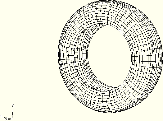
The model used in this analysis is essentially identical to that used in the first simulation discussed in “Symmetric results transfer for a static tire analysis,” Section 3.1.1, with CGAX4H and CGAX3H elements used in the axisymmetric model and rebar in the continuum elements for the belts and carcass. However, since no *STEADY STATE TRANSPORT steps are performed in this example, the TRANSPORT parameter is not needed during the symmetric model generation phase. In addition, instead of using a nonuniform discretization about the circumference, the uniform discretization shown in Figure 3.1.3–1 is used.
The incompressible hyperelastic material used to model the rubber includes a viscoelastic component described by a 1-term Prony series of the dimensionless shear relaxation modulus:
![]()
![]()
![]()
The loading sequence for computing the footprint solution is identical to that discussed in “Symmetric results transfer for a static tire analysis,” Section 3.1.1, with the axisymmetric model contained in tiredynamic_axi_half.inp, the partial three-dimensional model in tiredynamic_symmetric.inp, and the full three-dimensional model in tiredynamic_freqresp.inp. Since the NLGEOM=YES parameter is active for the *STATIC steps used in computing the footprint solution, the steady-state dynamic analyses, which are linear perturbation procedures, are performed about the nonlinear deformed shape of the footprint solution.
The first frequency response analyses of the tire are performed using the *STEADY STATE DYNAMICS, SUBSPACE PROJECTION option. The excitation is due to a harmonic vertical load of 200 N, which is applied to the analytical rigid surface through its reference node. The frequency is swept from 80 Hz to 130 Hz. The rim of the tire is held fixed throughout the analysis. Prior to the subspace analysis being performed, the eigenmodes that are used for the subspace projection are computed in a *FREQUENCY step. In the frequency step the first 20 eigenpairs are extracted, for which the computed eigenvalues range from 50 to 185 Hz.
The accuracy of the subspace analysis can be improved by including some of the stiffness associated with frequency-dependent material properties—i.e., viscoelasticity—in the eigenmode extraction step. This is accomplished by using the PROPERTY EVALUATION parameter with the *FREQUENCY option. In general, if the material response does not vary significantly over the frequency range of interest, the PROPERTY EVALUATION parameter can be set equal to the center of the frequency span. Otherwise, more accurate results will be obtained by running several separate frequency analyses over smaller frequency ranges with appropriate settings for the PROPERTY EVALUATION parameter. In this example a single frequency sweep is performed with PROPERTY EVALUATION=105 Hz.
The main advantage that the subspace projection method offers over mode-based techniques (“Mode-based steady-state dynamic analysis,” Section 6.3.8 of the ABAQUS Analysis User's Manual) is that it allows frequency-dependent material properties, such as viscoelasticity, to be included directly in the analysis. However, there is a cost involved in assembling the projected equations, and this cost must be taken into account when deciding between a subspace solution and a direct solution. ABAQUS offers four different parameter values that may be assigned to the SUBSPACE PROJECTION option to control how often the projected subspace equations are recomputed. These values are ALL FREQUENCIES, in which new projected equations are computed for every frequency in the analysis; EIGENFREQUENCY, in which projected equations are recomputed only at the eigenfrequencies; PROPERTY CHANGE, in which projected equations are recomputed when the stiffness and/or damping properties have changed by a user-specified percentage; and CONSTANT, which computes the projected equations only once at the center of the frequency range specified on the data lines of the *STEADY STATE DYNAMICS option. Setting SUBSPACE PROJECTION=ALL FREQUENCIES is, in general, the most accurate option; however, the computational overhead associated with recomputing the projected equations at every frequency can significantly reduce the cost benefit of the subspace method versus a direct solution. The SUBSPACE PROJECTION=CONSTANT option is the most inexpensive choice, but it should be chosen only when the material properties do not depend strongly on frequency. In general, the accuracy and cost associated with the four SUBSPACE PROJECTION parameter values are strongly problem dependent. In this example problem the results and computational expense for all four parameter values for SUBSPACE PROJECTION are discussed.
The results from the various subspace analyses are compared to the results from a *STEADY STATE DYNAMICS, DIRECT analysis.
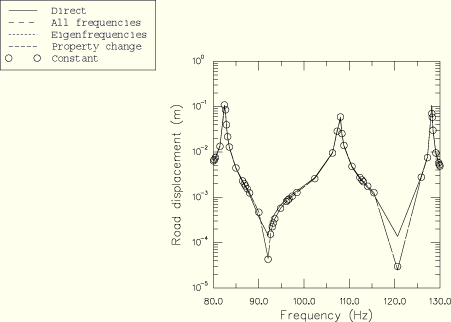
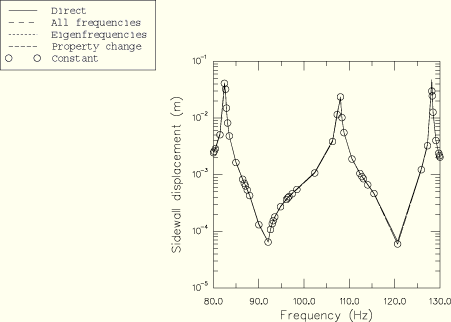
Each of the subspace analyses utilizes all 20 modes extracted in the *FREQUENCY step. Figure 3.1.3–2 shows the frequency response plots of the vertical displacements of the road's reference node for the direct solution along with the four subspace solutions using each of the SUBSPACE PROJECTION parameter values discussed above. Similarly, Figure 3.1.3–3 shows the frequency response plots of the horizontal displacement of a node on the tire's sidewall for the same five analyses. As illustrated in Figure 3.1.3–2 and Figure 3.1.3–3, all four of the subspace projection methods yield almost identical solutions; except for small discrepancies in the vertical displacements at 92 and 120 Hz, the subspace projection solutions closely match the direct solution as well. Timing results shown in Table 3.1.3–1 show that the SUBSPACE PROJECTION method results in savings in CPU time versus the direct solution.
Axisymmetric model, inflation analysis.
Partial three-dimensional model, footprint analysis.
Full three-dimensional model, steady-state dynamic analyses.
Axisymmetric model, inflation analysis with Marlow hyperelastic model.
Partial three-dimensional model, footprint analysis with Marlow hyperelastic model.
Full three-dimensional model, steady-state dynamic analyses with Marlow hyperelastic model.
Nodal coordinates for axisymmetric model.
Table 3.1.3–1 Comparison of normalized CPU times (normalized with respect to the DIRECT analysis) for the frequency sweep from 80 Hz to 130 Hz and the *FREQUENCY step.
| Normalized CPU time | |
|---|---|
| SUBSPACE PROJECTION=ALL FREQUENCIES | 0.89 |
| SUBSPACE PROJECTION=EIGENFREQUENCY | 0.54 |
| SUBSPACE PROJECTION=PROPERTY CHANGE | 0.49 |
| SUBSPACE PROJECTION=CONSTANT | 0.36 |
| DIRECT | 1.0 |
| *FREQUENCY | 0.073 |