
Product: ABAQUS/Explicit
The small-strain shell elements in ABAQUS/Explicit use a Mindlin-Reissner type of flexural theory that includes transverse shear and are based on a corotational velocity-strain formulation described by Belytschko et al. (1984, 1992). A corotational finite element formulation reduces the complexities of nonlinear mechanics by embedding a local coordinate system in each element at the sampling point of that element. By expressing the element kinematics in a local coordinate frame, the number of computations is reduced substantially. Therefore, the corotational velocity-strain formulation provides significant speed advantages in explicit time integration software, where element computations can dominate during the overall solution process.
The geometry of the shell is defined by its reference surface, which is determined by the nodal coordinates of the element. The embedded element corotational coordinate system, ![]() , is tangent to the reference surface and rotates with the element. This embedded corotational coordinate system serves as a local coordinate system and is constructed as follows:
, is tangent to the reference surface and rotates with the element. This embedded corotational coordinate system serves as a local coordinate system and is constructed as follows:
For the quadrilateral element the local coordinate ![]() is coincident with the line connecting the midpoints of sides,
is coincident with the line connecting the midpoints of sides, ![]() , as shown in Figure 3.6.6–1.
, as shown in Figure 3.6.6–1.
Figure 3.6.6–1 Local coordinate system for small-strain quadrilateral and triangular shell elements.
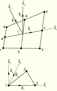
For the triangular element the local coordinate ![]() is coincident with the side connecting nodes 1 and 2 as shown in Figure 3.6.6–1. The
is coincident with the side connecting nodes 1 and 2 as shown in Figure 3.6.6–1. The ![]() –
–![]() plane coincides with the plane of the element.
plane coincides with the plane of the element.
Although the corotational coordinate system described here is used in the actual element computations, this system is transparent to the user. All reported stresses, strains, and other tensorial quantities for these shell elements are defined with respect to the coordinate system described in “Finite-strain shell element formulation,” Section 3.6.5.
The velocity of any point in the shell reference surface is given in terms of the discrete nodal velocity with the bilinear isoparametric shape functions ![]() as
as
![]()
![]()
In the Mindlin-Reissner theory of plates and shells, the velocity of any point in the shell is defined by the velocity of the reference surface, ![]() , and the angular velocity vector,
, and the angular velocity vector, ![]() , as
, as
![]()
![]()
![]()
![]()
![]()
![]()
![]()
The S4RS element is based on Belytschko et al. (1984). By using one-point quadrature at the center of the element—i.e., at ![]() =0—we obtain the gradient operator
=0—we obtain the gradient operator
![]()
The velocity strain can then be expressed as
![]()
![]()
![]()
![]()
![]()
![]()
The local nodal forces and moments are computed in terms of the section force and moment resultants by
![]()
![]()
![]()
![]()
![]()
![]()
![]()
![]()
The major objective in the development of the S4RS element was to obtain a convergent, stable element with the minimum number of computations. Because of the emphasis on speed, a few simplifications were made in formulating the equations for the S4RS element. Although the S4RS element performs very well in most practical applications, it has two known shortcomings:
It can perform poorly when warped, and in particular, it does not solve the twisted beam problem correctly.
It does not pass the bending patch test in the thin plate limit.
![]()
![]()
![]()
![]()
![]()
![]()
![]()
The components of the transverse shear velocity strain are given by
![]()
![]()
The angular velocity ![]() about outward facing vector
about outward facing vector ![]() is then given by a nodal projection
is then given by a nodal projection
![]()
![]()
![]()
Evaluating the resulting forms for the transverse shear at the centroidal quadrature point gives
![]()
![]()
![]()
![]()
![]()
The local nodal forces and moments are then given in terms of the section resultant forces and moments by
![]()
![]()
![]()
![]()
![]()
![]()
The triangular shell element formulation is similar to that of the S4RS element and is based on Kennedy et al. (1986). This element is not subject to zero energy modes inherent in quadrilateral element formulations.
The velocity strain is computed as in the S4RS element except that the gradient operator is given by
![]()
The local nodal forces and moments for the triangular shell can be expressed in terms of section resultant forces and moments as
![]()
![]()
![]()
![]()
![]()
The ![]() -components of the nodal forces are obtained by successively solving the following equations:
-components of the nodal forces are obtained by successively solving the following equations:
![]()
![]()
![]()
Since the one-point quadrature is used, several spurious modes, often known as hourglass modes, are possible for the quadrilateral elements. To suppress the hourglass modes, a consistent spurious mode control as described by Belytschko et al. (1984) is used. The hourglass shape vector ![]() is defined as
is defined as
![]()
![]()
![]()
![]()
![]()
![]()
![]()
![]()
The nodal hourglass forces and moments corresponding to the generalized hourglass stresses are
![]()
![]()
![]()
