Products: ABAQUS/Standard ABAQUS/Explicit
This section describes the formulation of the quadrilateral finite-membrane-strain element S4R, the triangular element S3R and S3 obtained through degeneration of S4R, and the fully integrated finite-membrane-strain element S4.
At a given stage in the deformation history of the shell, the position of a material point in the shell is defined by
![]()
![]()
In the deformed state we define local, orthonormal shell directions ![]() such that
such that
![]()
![]()
![]()
![]()
In the original (reference) configuration we denote the position by ![]() (
(![]() for the reference surface) and the direction vectors by
for the reference surface) and the direction vectors by ![]() , which yields
, which yields
![]()
![]()
![]()
![]()
![]()
The position of the points in the shell reference surface is described in terms of discrete nodal positions with parametric interpolation functions ![]() . The functions are
. The functions are ![]() continuous, and
continuous, and ![]() are nonorthogonal, nondistance measuring parametric coordinates. For the reference surface positions one, thus, obtains
are nonorthogonal, nondistance measuring parametric coordinates. For the reference surface positions one, thus, obtains
![]()
![]()
Now consider the original configuration. The unit normal to the shell reference surface is readily obtained as
![]()
![]()
![]()
![]()
![]()
It is convenient to define the inverse of the reference surface deformation gradient
![]()
![]()
![]()
![]()
![]()
![]()
![]()
![]()
![]()
The equations given in the earlier sections are valid for any local coordinate system defined in the current state. The ![]() vectors at the beginning of the analysis are determined following the standard ABAQUS conventions. In this section, we outline the way in which the in-plane coordinates are made corotational.
vectors at the beginning of the analysis are determined following the standard ABAQUS conventions. In this section, we outline the way in which the in-plane coordinates are made corotational.
To obtain the updated version of ![]() , we follow a two-step approach. First, we construct orthogonal vectors
, we follow a two-step approach. First, we construct orthogonal vectors ![]() tangential to the surface (following ABAQUS conventions). Subsequently, we calculate
tangential to the surface (following ABAQUS conventions). Subsequently, we calculate
![]()
![]()
![]()
![]()
![]()
![]()
We assume that the nodal spin will be interpolated with the interpolation functions ![]() . During an increment the nodal spin is assumed to be constant; consequently, the value of the spin at each material point will be constant. Hence, we can use the same interpolation functions for the incremental finite rotation vector
. During an increment the nodal spin is assumed to be constant; consequently, the value of the spin at each material point will be constant. Hence, we can use the same interpolation functions for the incremental finite rotation vector ![]() :
:
![]()
![]()
![]()
![]()
![]()
![]()
![]()
![]()
![]()
![]()
![]()
For the gradient ![]() of the updated shell normal we obtain
of the updated shell normal we obtain
![]()
Calculation of ![]() involves taking the gradient with respect to the reference configuration. It is more convenient to use the reference surface curvature tensor
involves taking the gradient with respect to the reference configuration. It is more convenient to use the reference surface curvature tensor
![]()
![]()
![]()
We already have obtained an expression for the deformation gradient in the reference surface, and we have assumed that the thickness change is constant:
![]()
![]()
![]()
![]()
The membrane strain increment follows from the incremental stretch tensor ![]() , whose components follow from the incremental deformation gradient
, whose components follow from the incremental deformation gradient ![]() by the polar decomposition
by the polar decomposition ![]() .
.
Let ![]() and
and ![]() be the deformation gradient at the beginning and the end of the increment, respectively. By definition
be the deformation gradient at the beginning and the end of the increment, respectively. By definition ![]() . The incremental deformation gradient follows as
. The incremental deformation gradient follows as
![]()
![]()
Following Koiter-Sanders shell theory, and compensating for the rotation of the base vectors relative to the material, we define the physical curvature increment ![]() as
as
![]()
![]()
![]()
![]()
The virtual work contribution of the stresses is
![]()
![]()
![]()
![]()
![]()
![]()
The variation in the curvature is obtained by taking variations in the incremental curvature, which yields
![]()
![]()
![]()
![]()
To obtain an expression for the rate of virtual work, we first write the virtual work equation in terms of the reference volume
![]()
![]()
![]()
![]()
![]()
It remains to determine ![]() and
and ![]() . From the first variation
. From the first variation ![]() follows
follows
![]()
![]()
![]()
![]()
![]()
We need to calculate the second variation of the curvature to calculate the initial stress contribution from the curvature:
![]()
![]()
Denoting derivatives with respect to the isoparametric coordinates as ![]() , the second variation of the curvature is
, the second variation of the curvature is
![]()
Several interpolation schemes have been proposed to avoid shear-locking, which typically arises as the thickness of a plate or shell goes to zero. Here we employ an assumed strain method based on the Hu-Washizu principle. This scheme derives from that by MacNeal (1978), subsequently extended and reformulated in Hughes and Tezduyar (1981) and MacNeal (1982) and revisited in Bathe and Dvorkin (1984). Computational aspects of the nonlinear theory are investigated in Simo, Fox, and Rifai (1989) for fully integrated quadrilateral shell elements. For reduced integration quadrilateral and triangular shell elements that can be used for both implicit and explicit integration, this assumed strain method needs to be modified. We summarize below the assumed strain method used with fully integrated elements, followed by the modifications required for the one-point integration plus stabilization used in ABAQUS.
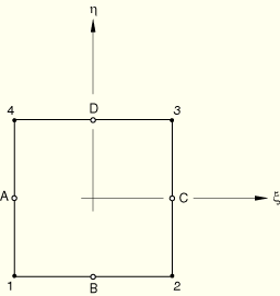
Consider a typical isoparametric finite element, as depicted in Figure 3.6.5–1, and denote by ![]() the set of midpoints of the element boundaries.
the set of midpoints of the element boundaries.
The following assumed transverse shear strain field is used:
By making use of the assumed strain field along with the update formulae for the director field, the assumed covariant transverse shear field can be written concisely in matrix notation. Recall the director field update equation and the corresponding linearized director field:
![]()
![]()
![]()
![]()
A St. Venant-Kirchhoff constitutive model for the Kirchhoff curvilinear components of the resultant transverse shear force is written in terms of the transverse shear strains as
![]()
![]()
![]()
![]()
The calculation of the initial stress stiffness matrix requires the second variation of the assumed transverse strain field. This calculation can be summarized in matrix notation as follows. Define vectors of variations of the nodal displacement quantities:
![]()
For reduced-integration elements the transverse shear force components need to be evaluated at the center of the elements. Consider ![]() the transverse shear contribution to the internal energy:
the transverse shear contribution to the internal energy:
![]()
This transverse shear energy can be approximated in many ways to produce a one point integration at the center of the element plus hourglass stabilization. It is important that this treatment yield accurate representation of transverse shear deformation in thick shell problems and provide robust performance for skewed elements. The treatment should collapse smoothly to a triangle, which should be insensitive to the node numbering during collapse; that is, the triangle's response should not depend on the nodal connectivity. For an entire mesh of triangular elements, the treatment should give convergent results (that is, the element should not lock). Furthermore, the high frequency response of the transverse shear treatment should be controlled so that transverse shear response does not dominate the stable time increment for explicit dynamic analysis (including for skewed triangular or quadrilateral geometries). All of these requirements are embodied in the following transverse shear treatment.
Define the transverse shear strain at the center of the element (the homogeneous part) and the “hourglass” transverse shear strain vectors as
![]()
![]()
The inclusion of the crop circle strain ![]() in the homogeneous part of the transverse shear strain
in the homogeneous part of the transverse shear strain ![]() has two important consequences. First, it makes the transverse shear response insensitive to the nodal connectivity for a triangular element. That is, when a side of a quadrilateral element is collapsed to form a triangle, the element's response is independent of the choice of node numbering on the element. Second, for explicit dynamic analyses the coefficients
has two important consequences. First, it makes the transverse shear response insensitive to the nodal connectivity for a triangular element. That is, when a side of a quadrilateral element is collapsed to form a triangle, the element's response is independent of the choice of node numbering on the element. Second, for explicit dynamic analyses the coefficients ![]() and
and ![]() are chosen to minimize the highest frequencies associated with the homogeneous part of the transverse shear response.
are chosen to minimize the highest frequencies associated with the homogeneous part of the transverse shear response.
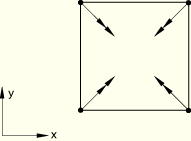
To illustrate the crop circle and butterfly transverse shear patterns, consider a square, initially flat element. Furthermore, consider plate theory kinematics; that is, two rotations and a vertical deflection at the nodes. The crop circle pattern has zero vertical deflection at the nodes and a nodal rotation vector pattern as illustrated in Figure 3.6.5–2.
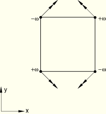
The butterfly pattern has vertical deflections that correspond to cross-diagonal bending; that is, two equal deflections at two nodes across a diagonal, with equal and opposite deflections at the remaining two nodes. The nodal rotations develop in a way that opposes the bending motion of the reference surface; that is, the rotations are opposite the rotations that would develop for this displacement pattern to produce pure bending. The butterfly mode's nodal vertical deflection and rotation vector pattern are illustrated in Figure 3.6.5–3.Let the reference element area be![]()
![]()
The formulation of the homogeneous part of the transverse shear has two contributions: the average edge strain across the element, plus the element distortion term. The average strain treatment is essentially the same as that for the assumed strain formulation of MacNeal and others presented earlier, with expressions evaluated at the center of the element (![]() and
and ![]() ). The details of this part are omitted; only the element distortion term is presented in detail. The variation of the homogeneous transverse shear strain can be written
). The details of this part are omitted; only the element distortion term is presented in detail. The variation of the homogeneous transverse shear strain can be written
![]()
![]()
![]()
The stabilization term has a similar formulation. The variation of the hourglass strain is
![]()
![]()
![]()
The hourglass force components ![]() and
and ![]() are given by the constitutive relations
are given by the constitutive relations
![]()
(1) The butterfly mode ![]() is applied with a “large” or physical hourglass stiffness. For a reference geometry with constant Jacobian, the butterfly stabilization term can be derived from an exact integration of the assumed strain formulation of the transverse shear energy. It is important to apply this constraint with a high stiffness to prevent overly flexible response for quadrilateral elements. The crop circle mode is applied with a “small” or weak stiffness. Although this mode can propagate, it is rarely problematic and is often prevented with boundary conditions.
is applied with a “large” or physical hourglass stiffness. For a reference geometry with constant Jacobian, the butterfly stabilization term can be derived from an exact integration of the assumed strain formulation of the transverse shear energy. It is important to apply this constraint with a high stiffness to prevent overly flexible response for quadrilateral elements. The crop circle mode is applied with a “small” or weak stiffness. Although this mode can propagate, it is rarely problematic and is often prevented with boundary conditions.
(2) As the quadrilateral element is degenerated to a triangle, the two hourglass constraints converge into a single constraint: the crop circle constraint. However, as is well-known, for a constant strain triangle the element will lock for certain meshes with three transverse shear constraints per element. Therefore, in the case of a triangular element, the (strong) butterfly mode stabilization is not applied. Only the (weak) crop circle mode stabilization is applied. Thus, in addition to the two homogeneous transverse shear strains, the triangle has a weak constraint to prevent spurious zero energy modes, yet avoids locking in most situations.
The initial stress contribution from the stabilization terms takes the following form:
![]()

The initial stress contribution from the homogeneous part consists of two terms, one from the assumed strain formulation (evaluated at ![]() ) as detailed earlier, and the other from the crop circle mode addition. These two terms can be written
) as detailed earlier, and the other from the crop circle mode addition. These two terms can be written
![]()
The in-plane displacement hourglass control is applied in the same way as in the ABAQUS membrane elements. The hourglass strains are defined by
![]()
![]()
![]()
![]()
![]()
![]()
![]()
![]()
![]()
![]()
The expressions for the curvature change, the transverse shear constraints, and the drilling mode constraints still leave three nonhomogeneous rotational modes unconstrained. These modes correspond to zero rotation at the midedges and zero gradient at the centroid. Hence, they correspond to the familiar ![]() hourglass pattern. To pass curvature patch tests exactly, it is necessary to use orthogonalized hourglass patterns as derived for in-plane hourglass control.
hourglass pattern. To pass curvature patch tests exactly, it is necessary to use orthogonalized hourglass patterns as derived for in-plane hourglass control.
This last aspect implies that the rotational hourglass mode corresponds to the mixed derivative of the rotation at the centroid:
![]()
We cannot use the above formulation directly in a formulation suitable for multiple finite rotation increments. Hence, we use the same approach as for the calculation of the curvature change. For the purpose of the calculation we define the updated shell direction vectors
![]()
![]()
![]()
![]()
![]()
![]()
![]()
![]()
![]()
![]()
![]()
![]()
![]()
![]()
![]()
![]()
![]()
In general meshes it will be desirable to collapse at least some of the quadrilateral elements to triangles or to use the triangular element S3 or S3R, which is in fact an internally collapsed S4R element. For this case the calculation of the membrane strains and the curvature changes proceeds along the same lines as before. The transverse shears will now be zero at the degenerate edges. Finally, calculation of all hourglass constraints will be omitted.
For numerical efficiency in explicit dynamic analysis, it is desirable to have the stable time increment determined by the membrane response of the structure. For this reason scaling of the rotary inertia based on the element's reference geometry is included in ABAQUS/Explicit.
In explicit dynamic analyses the stable time increment is proportional to the inverse of the highest frequency of the element. Therefore, we must ensure that the highest frequency associated with the transverse shear response does not exceed the highest frequency associated with the membrane response. For thick elements (that is, for elements whose thickness is order unity relative to a characteristic length in the element), the membrane frequencies are dominant. The primary consideration in choosing appropriate scalings is that in the limit as the element's thickness goes to zero, the transverse shear frequencies remain below the membrane ones. Recall that for a one-dimensional spring-mass oscillator, the natural frequency ![]() can be written in terms of the stiffness
can be written in terms of the stiffness ![]() and the mass
and the mass ![]() as
as
![]()
For thin elements the rotary inertia is small (negligible) relative to the rotational inertia of the mass at the nodes rotating about an axis through the element center. Therefore, we choose a scaling on the rotary inertia such that it never becomes smaller than a fixed (small) percentage of the rotational inertia of the mass at the nodes rotating about an axis through the center of the element.
Let ![]() be the nondimensional rotary inertia scaling, where
be the nondimensional rotary inertia scaling, where ![]() . When
. When ![]() , the true rotary inertia is used. Consider a lumped mass matrix for a 4-node element, and let the element be flat and square. For rotations about an axis in the plane of the element, parallel to an element edge, passing through the center, the contribution to the rotational inertia of the mass at the nodes is
, the true rotary inertia is used. Consider a lumped mass matrix for a 4-node element, and let the element be flat and square. For rotations about an axis in the plane of the element, parallel to an element edge, passing through the center, the contribution to the rotational inertia of the mass at the nodes is
![]()
![]()
![]()
![]()
For planar geometries with element directors along the normal direction, closed-form expressions are possible for the highest membrane and transverse shear frequencies. In such cases the length parameter ![]() is interpreted as a characteristic element length that depends on the element distortion. To handle arbitrarily shaped curved elements, exact calculation of the element frequencies becomes difficult. However, we can safely bound the frequencies by an appropriate choice of
is interpreted as a characteristic element length that depends on the element distortion. To handle arbitrarily shaped curved elements, exact calculation of the element frequencies becomes difficult. However, we can safely bound the frequencies by an appropriate choice of ![]() in the following scaling:
in the following scaling:
![]()
For the displacement degrees of freedom, bulk viscosity introduces damping associated with volumetric straining. Linear bulk viscosity or truncation frequency damping is used to damp the high frequency ringing that leads to unwanted noise in the solution or spurious overshoot in the response amplitude. For the same reason, in shells we need to damp the high frequency ringing in the rotational degrees of freedom with linear bulk viscosity acting on the mean curvature strain rate. This damping generates a bulk viscosity “pressure moment,” ![]() , which is linear in the mean curvature strain rate:
, which is linear in the mean curvature strain rate:
![]()
Element S4 is a fully integrated finite-membrane-strain shell element. Since the element's stiffness is fully integrated, no spurious membrane or bending zero energy modes exist and no membrane or bending mode hourglass stabilization is used. Drill rotation control, however, is required. Element S4 uses the same drill stiffness formulation as used for element S4R. Similarly, element S4 assumes that the transverse shear strain (and force, since the transverse shear treatment is elastic based on the initial elastic modulus of the material) is constant over the element. Therefore, all four stiffness integration locations will have the same transverse shear strain, transverse shear section force, and transverse shear stress distribution. The transverse shear treatment for S4 is identical to that for S4R.
It is well known that a standard displacement formulation will exhibit shear locking for applications dominated by in-plane bending deformation. However, a standard displacement formulation for the out-of-plane bending stiffness is not subject to similar locking response. Hence, S4 uses a standard displacement formulation for the element's bending stiffness, and the theory presented above for the rotation kinematics and bending strain measures applies to S4. The primary difference between the element formulations for S4 and S4R is the treatment of the membrane strain field. This formulation is the topic of the following discussion.
The membrane formulation used for S4 does not rely on the fact that S4 is a shell element. Hence, the discussion below details the formulation from the point of view that the membrane response is governed by the equilibrium for a three-dimensional body in a state of plane stress.
Consider an enhancement ![]() to the rate of deformation tensor
to the rate of deformation tensor ![]() . We introduce the enhanced rate of deformation tensor,
. We introduce the enhanced rate of deformation tensor, ![]() , as
, as
![]()
Admissible variations in the rate of deformation are also introduced as
![]()
![]()
We now introduce constraints on the enhancements ![]() and
and ![]() :
:
![]()
![]()
In the modified virtual work statement all kinematic quantities and corresponding variations (![]() ,
, ![]() ,
, ![]() , and
, and ![]() ) are known functions of
) are known functions of ![]() ,
, ![]() , and the reference configuration. A fundamental requirement for the validity of the formulation is that the modified virtual work statement leads to the proper equilibrium equations. If
, and the reference configuration. A fundamental requirement for the validity of the formulation is that the modified virtual work statement leads to the proper equilibrium equations. If ![]() is arbitrary, the constraint equations can be rewritten as
is arbitrary, the constraint equations can be rewritten as
![]()
![]()
In the actual implementation we choose to satisfy the constraints only for piecewise constant stress fields ![]() . Hence, over the element domain
. Hence, over the element domain ![]() we require
we require
![]()
To pass the patch test, the choice of enhancements ![]() cannot be arbitrary. A sufficient condition for the satisfaction of the patch test is that for homogeneous deformations we have
cannot be arbitrary. A sufficient condition for the satisfaction of the patch test is that for homogeneous deformations we have ![]() or
or ![]() pointwise. In that case
pointwise. In that case ![]() and the stress is homogeneous. Since the stress is homogeneous, it can be moved outside the volume integral in the modified virtual work statement. The volume integral condition on
and the stress is homogeneous. Since the stress is homogeneous, it can be moved outside the volume integral in the modified virtual work statement. The volume integral condition on ![]() implies that the expression is independent of the enhancement and leads to the standard displacement formulation, which is known to satisfy the patch test.
implies that the expression is independent of the enhancement and leads to the standard displacement formulation, which is known to satisfy the patch test.