You have been asked to investigate what happens if the steel connecting lug from Chapter 4, “Using Continuum Elements,” is subjected to an extreme load (60 kN) caused by an accident. The results from the linear analysis indicate that the lug will yield. You need to determine the extent of the plastic deformation in the lug and the magnitude of the plastic strains, so that you can assess whether or not the lug will fail.
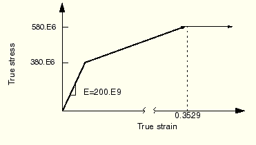
The only inelastic material data available for the steel are its yield stress (380 MPa) and its strain at failure (0.15). You decide to assume that the steel is perfectly plastic: the material does not harden, and the stress can never exceed 380 MPa (see Figure 8–6).
In reality some hardening will probably occur, but this assumption is conservative; if the material hardens, the plastic strains will be less than those predicted by the simulation.Copy the existing input file, lug.inp, to a new file, lug_plas.inp. Modify this file to include the changes described below. If you wish to create the entire model using ABAQUS/CAE please refer to “Example: connecting lug with plasticity,” Section 10.4 of Getting Started with ABAQUS.
Specify the post-yield behavior of the material using the *PLASTIC option. The Young's modulus for the material is 200 GPa, and the initial yield stress at zero plastic strain is 380 MPa. Since you are modeling the steel as perfectly plastic, no other yield stresses are given on the *PLASTIC option.
The complete material definition is, therefore:
*MATERIAL, NAME=STEEL
*ELASTIC
200.E9, 0.3
*PLASTIC
380.E6,0.0
All other option blocks in the model definition portion of the input file remain unchanged.
You must perform a general, nonlinear simulation because of the nonlinear material behavior in the model. Therefore, you must remove the PERTURBATION parameter from the *STEP option. Set the total step time in the *STATIC procedure option block to 1.0. Use an initial increment size that is 20% of the total step time. This simulation is a static analysis of the lug under the extreme loads; you do not know in advance how many increments this simulation may require. The default maximum of 100 increments, however, is reasonably large and should be sufficient for this analysis. Also, assume that the effects of geometric nonlinearity will not be important in this simulation, so omit the NLGEOM parameter from the *STEP option. These modifications to your input file should look like:
*STEP
*STATIC
0.2,1.0
Loading
The load applied in this simulation is twice what was applied in the linear elastic simulation of the lug (60 kN vs. 30 kN). Therefore, double the magnitude of the pressures applied to the lug. The modified *DLOAD option block in your model will look similar to the following:
*DLOAD
PRESS, P6, 1.E+08
Output requests
You will use ABAQUS/Viewer to review all of the results from this simulation, so suppress all printed output requests by setting the FREQUENCY parameter equal to zero. The output request options in your input file should look similar to those shown below:
*NODE PRINT, FREQUENCY=0
*EL PRINT, FREQUENCY=0
*OUTPUT, FIELD, FREQUENCY=1, VARIABLE=PRESELECT
You will need to save some history data in the output database file to use with the X–Y plotting capability in ABAQUS/Viewer. Store the displacements for node set HOLEBOT, which should already exist, using the following option:
*OUTPUT, HISTORY, FREQUENCY=1
*NODE OUTPUT, NSET=HOLEBOT
U,
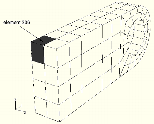
You also want detailed results for one of the elements along the built-in end of the lug (see Figure 8–7).
This is element 206 in the mesh generated by the commands found in “Connecting lug with plasticity,” Section A.6; the element in this location may have a different number in your model. This element is chosen because it is the element for which the stresses are most likely to be largest in magnitude. Create an element set that contains the element, and save the stresses (S), stress invariants (SINV), plastic strains (PE), and strains (E) for that element set in the output database file. The necessary option blocks are shown below:*ELEMENT OUTPUT, ELSET=EL206 S, SINV, PE, E *ELSET, ELSET=EL206 206,
Save these changes to your model, and run the analysis with the following command:
abaqus job=lug_plas
Status file
Monitor the simulation while it is running by looking at the status file, lug_plas.sta. When ABAQUS has finished the simulation, your status file will contain information similar to the following:
SUMMARY OF JOB INFORMATION:
 STEP  INC ATT SEVERE EQUIL TOTAL  TOTAL      STEP       INC OF       DOF    IF
               DISCON ITERS ITERS  TIME/    TIME/LPF    TIME/LPF    MONITOR RIKS
               ITERS               FREQ
   1     1   1     0     1     1  0.200      0.200      0.2000
   1     2   1     0     1     1  0.400      0.400      0.2000
   1     3   1     0     3     3  0.700      0.700      0.3000
   1     4   2     0     2     2  0.775      0.775      0.07500
   1     5   1     0     4     4  0.887      0.887      0.1125
   1     6   2     0     3     3  0.916      0.916      0.02813
   1     7   2     0     2     2  0.926      0.926      0.01055
   1     8   1     0     4     4  0.942      0.942      0.01582
   1     9   2     0     5     5  0.948      0.948      0.005933
   1    10   2     0     4     4  0.949      0.949      0.001483
   1    11   1     0     4     4  0.951      0.951      0.001483
   1    12   2     0     3     3  0.951      0.951      0.0005562
   1    13   1     0     4     4  0.952      0.952      0.0008343
   1    14   2     0     4     4  0.953      0.953      0.0003129
   1    15   2     0     3     3  0.953      0.953      0.0001173
   1    16   2     0     3     3  0.953      0.953      4.399e-05
   1    17   1     0     3     3  0.953      0.953      6.599e-05
   1    18   2     0     2     2  0.953      0.953      2.475e-05
   1    19   1     0     3     3  0.953      0.953      3.712e-05
   1    20   2     0     3     3  0.953      0.953      1.392e-05
   1    21   1     0     3     3  0.953      0.953      2.088e-05
   1    22   2     0     2     2  0.953      0.953      1.000e-05
   1    23   1     0     3     3  0.953      0.953      1.500e-05
   1    24   2     0     2     2  0.953      0.953      1.000e-05
ABAQUS was able to apply only 95% of the prescribed load to the model and still obtain a converged solution. The status file shows that ABAQUS reduced the size of the time increment, which is shown in the last (right-hand) column, many times during the simulation and stopped the analysis in the 24th increment. You will have to look at the information in the message file to understand why ABAQUS terminated the simulation early.Message file
The message file, lug_plas.msg, contains detailed information about the simulation's progress (see “Results,” Section 7.4.3, for more information about the format of the message file).
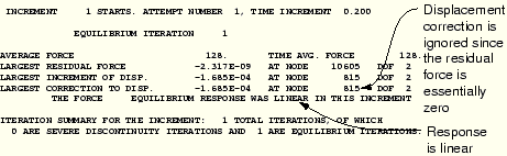
Look at the information for the first increment in the analysis (it is also shown below); you will discover that the model's initial behavior is linear. The model's behavior was also linear in the second increment.
ABAQUS requires several iterations to obtain a converged solution in the third increment, which indicates that nonlinear behavior occurred in the model during this increment. The only nonlinearity in the model is the plastic material behavior, so the steel must have started to yield somewhere in the lug at this applied load magnitude. The summaries of the iterations for the third increment are shown below.
INCREMENT 3 STARTS. ATTEMPT NUMBER 1, TIME INCREMENT 0.300
EQUILIBRIUM ITERATION 1
AVERAGE FORCE 450. TIME AVG. FORCE 278.
LARGEST RESIDUAL FORCE -524. AT NODE 13041 DOF 1
LARGEST INCREMENT OF DISP. -2.545E-04 AT NODE 815 DOF 2
LARGEST CORRECTION TO DISP. -1.800E-06 AT NODE 10817 DOF 2
FORCE EQUILIBRIUM NOT ACHIEVED WITHIN TOLERANCE.
EQUILIBRIUM ITERATION 2
AVERAGE FORCE 451. TIME AVG. FORCE 279.
LARGEST RESIDUAL FORCE -1.71 AT NODE 23041 DOF 3
LARGEST INCREMENT OF DISP. -2.576E-04 AT NODE 815 DOF 2
LARGEST CORRECTION TO DISP. -3.140E-06 AT NODE 10817 DOF 2
FORCE EQUILIBRIUM NOT ACHIEVED WITHIN TOLERANCE.
EQUILIBRIUM ITERATION 3
AVERAGE FORCE 451. TIME AVG. FORCE 279.
LARGEST RESIDUAL FORCE 1.174E-04 AT NODE 3041 DOF 3
LARGEST INCREMENT OF DISP. -2.576E-04 AT NODE 20815 DOF 2
LARGEST CORRECTION TO DISP. -4.469E-09 AT NODE 817 DOF 2
THE FORCE EQUILIBRIUM EQUATIONS HAVE CONVERGED
ITERATION SUMMARY FOR THE INCREMENT: 3 TOTAL ITERATIONS, OF WHICH
0 ARE SEVERE DISCONTINUITY ITERATIONS AND 3 ARE EQUILIBRIUM ITERATIONS.
TIME INCREMENT COMPLETED 0.300 , FRACTION OF STEP COMPLETED 0.700
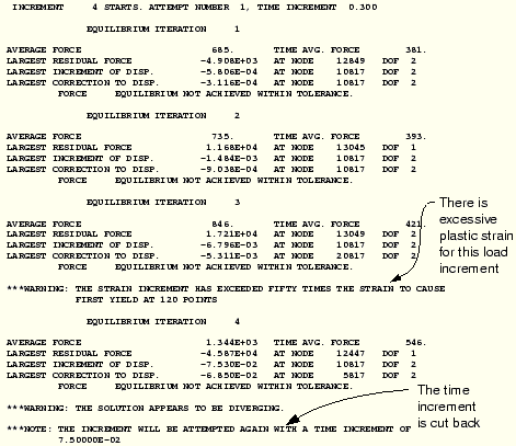
STEP TIME COMPLETED 0.700 , TOTAL TIME COMPLETED 0.700ABAQUS attempts to find a solution in the fourth increment using an increment size of 0.3, which means it is applying 30% of the total load, or 18 MPa, during this increment. After several iterations, ABAQUS issues warning messages that the strain increments it calculated exceed the strain at initial yield by 50 times. After a few more iterations ABAQUS determines that the solution in this increment is not going to converge; instead, it is diverging. Therefore, ABAQUS abandons this attempt at finding a solution, reduces the increment size to 25% of the value used in the first attempt, and tries a second attempt at finding a solution. This reduction in increment size is called a cut-back. With the smaller increment size, ABAQUS finds a converged solution in just a few iterations. Some of the iteration summaries from the first attempt of the fourth increment are shown below.
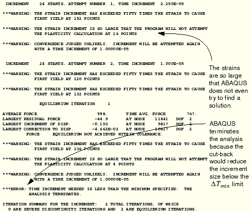
Now that you have reviewed the early increments of the simulation, move to the end of the message file and review the last increment ABAQUS attempted. You will see that ABAQUS is using a very small increment size, on the order of 1.0 × 10⁻⁵, in this final increment because of the many cut-backs. The iteration summaries for the last increment are shown below. ABAQUS makes two attempts to find a solution in this final increment, but it must cut back the time increment in each attempt because the strain increments are so large that it does not even try to perform the plasticity calculations. This check on the magnitude of the total strain increment is another example of the many automatic solution controls ABAQUS uses to ensure that the solution obtained for your simulation is both accurate and efficient. The automatic solution controls are suitable for almost all simulations. Therefore, you do not have to worry about providing parameters to control the solution algorithm: you only have to be concerned with the input data for your model.
If you look at the summary at the end of the message file, you will find that ABAQUS issued many warning messages during the analysis. Reviewing the message file will show that most of these warnings were the result of numerical problems with the plasticity calculations. You know that ABAQUS terminated the analysis early because these numerical problems forced it to cut back the time increment until it was below the minimum allowable time increment.
In the third column of the status file you will see the number of attempts ABAQUS made to solve an increment. In the sixth column the number of iterations needed for the last attempt at an increment is printed. Now, you should look at the results in ABAQUS/Viewer to understand what caused this excessive plasticity.
Run ABAQUS/Viewer by entering the following command:
abaqus viewer odb=lug_plasat the operating system prompt.
Plotting the deformed model shape
Create a plot of the model's deformed shape, and check that this shape is realistic. Do not include the undeformed model shape in the plot.
From the main menu bar, select Plot![]() Deformed Shape; or use the
Deformed Shape; or use the ![]() tool in the toolbox. ABAQUS/Viewer displays the plot shown in Figure 8–8.
tool in the toolbox. ABAQUS/Viewer displays the plot shown in Figure 8–8.
The default view is isometric. You can set the view shown in Figure 8–8 by using the options in the View menu or the view tools in the toolbar. The displacements and, particularly, the rotations of the lug shown in the plot are large. Yet they do not seem large enough to have caused all of the numerical problems seen in the simulation. Look closely at the information in the plot's title for an explanation. The deformation scale factor ABAQUS/Viewer used in this plot was 0.02; the displacements are scaled to 2% of their actual values.
ABAQUS/Viewer always scales the displacements in a geometrically linear simulation such that the deformed shape of the model fits into the viewport. (This is in contrast to a geometrically nonlinear simulation, where ABAQUS/Viewer does not scale the displacements and, instead, adjusts the view by zooming in or out to fit the deformed shape in the plot.) If you want to plot the actual displacements, you must set the deformation scale factor to 1.0.
To set the deformation scale factor:
From the main menu bar, select Options![]() Deformed Shape.
Deformed Shape.
The Deformed Shape Plot Options dialog box appears.
In the Deformation Scale Factor area, toggle on Uniform and enter 1.0 in the Value text field that appears.
Click OK to apply your selection and to close the dialog box.
This will produce a plot of the model in which the lug has rotated until it is almost parallel to the vertical (global Y) axis.
The applied load of 60 kN exceeds the limit load of the lug, and the lug collapses when the material yields at all of the integration points through its thickness. The lug then has no stiffness to resist further deformation because of the perfectly plastic post-yield behavior of the steel.
The ABAQUS connecting lug simulation with perfectly plastic material behavior predicts that the lug will suffer catastrophic failure caused by the collapse of the structure. We have already mentioned that the steel would probably exhibit some hardening after it has yielded. You suspect that including hardening behavior would allow the lug to withstand this 60 kN load because of the additional stiffness it would provide. Therefore, you decide to add some hardening to the steel's material property definition. Assume that the yield stress increases to 580 MPa at a plastic strain of 0.35, which represents typical hardening for this class of steel. The stress-strain curve for the modified material model is shown in Figure 8–9. Modify your *PLASTIC option block as follows so that it includes the hardening data:
*PLASTIC
380.E6, 0.00
580.E6, 0.35
Save the model with plastic hardening to a new input file named lug_plas_hard.inp, and run the analysis using the command
abaqus job=lug_plas_hard
Status file
The summary of the analysis in the status file, which is shown below, shows that ABAQUS found a converged solution when the full 60 kN load was applied. The hardening data added enough stiffness to the lug to prevent it from collapsing under the 60 kN load.
 SUMMARY OF JOB INFORMATION:
 STEP  INC ATT SEVERE EQUIL TOTAL  TOTAL      STEP       INC OF       DOF    IF
               DISCON ITERS ITERS  TIME/    TIME/LPF    TIME/LPF    MONITOR RIKS
               ITERS               FREQ
   1     1   1     0     1     1  0.200      0.200      0.2000
   1     2   1     0     1     1  0.400      0.400      0.2000
   1     3   1     0     3     3  0.700      0.700      0.3000
   1     4   1     0     7     7  1.00       1.00       0.3000
In this simulation there is very little information of interest in the message file. There are no warnings issued during the analysis, so you can proceed directly to postprocessing the results with ABAQUS/Viewer.
Start ABAQUS/Viewer, and use the following command to review the results of the second analysis:
abaqus viewer odb=lug_plas_hard
Deformed model shape and peak displacements
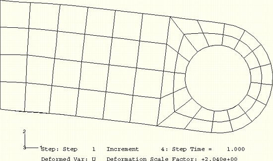
Plot the deformed model shape with these new results. It should look similar to the plot shown in Figure 8–10. The default deformation scale factor in this plot is 2.04, making the displayed deformations roughly double the actual deformations.
Contour plot of Mises stress
Contour the Mises stress in the model. Create a filled contour plot on the actual deformed shape of the lug with the plot title suppressed.
To contour the Mises stress:
From the main menu bar, select Result![]() Field Output.
Field Output.
The Field Output dialog box appears; by default, the Primary Variable tab is selected.
From the list of output variables, select S.
From the list of invariants, select Mises.
Click OK.
The Select Plot Mode dialog box appears.
Toggle on Contour, and click OK.
ABAQUS/Viewer displays a contour plot of the Mises stress.
You will set the deformation scale factor to produce the plot shown in Figure 8–11.
Click Contour Options in the prompt area.
ABAQUS/Viewer displays the Contour Plot Options dialog box.
Click the Shape tab, select the Uniform deformation scale factor, and set its value to 1.0.
Click the Basic tab and drag the uniform contour intervals slider to 10.
Click OK to view the contour plot and to close the Contour Plot Options dialog box.
The contour plot title is displayed by default but can be turned off.
To suppress the plot title and state blocks, select Viewport![]() Viewport Annotation Options.
Viewport Annotation Options.
The Viewport Annotation Options dialog box appears.
Click the General tab, and toggle off Show title block and Show state block.
Click OK to apply your selections and to close the dialog box.
The customized contour plot appears.
Use the view manipulation tools to position and size the model to obtain a plot similar to that shown in Figure 8–11.
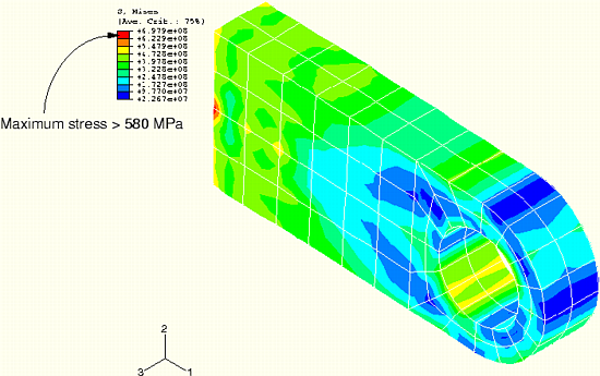
Do the values listed in the contour legend surprise you? The maximum stress is greater than 580 MPa, which should not be possible since the material was assumed to be perfectly plastic at this stress magnitude. This misleading result occurs because of the algorithm that ABAQUS/Viewer uses to create contour plots for element variables, such as stress. The contouring algorithm requires data at the nodes; however, ABAQUS/Standard calculates element variables at the integration points. ABAQUS/Viewer calculates nodal values of element variables by extrapolating the data from the integration points to the nodes. The extrapolation order depends on the element type; for second-order, reduced-integration elements ABAQUS/Viewer uses linear extrapolation to calculate the nodal values of element variables. To display a contour plot of Mises stress, ABAQUS/Viewer extrapolates the stress components from the integration points to the nodal locations within each element and calculates the Mises stress. If the differences in Mises stress values fall within the specified averaging threshold, nodal averaged Mises stresses are calculated from each surrounding element's invariant stress value. Invariant values exceeding the elastic limit can be produced by the extrapolation process.
Try plotting contours of each component of the stress tensor (variables S11, S22, S33, S12, S23, and S13). You will see that there are significant variations in these stresses across the elements at the built-in end. This causes the extrapolated nodal stresses to be higher than the values at the integration points. The Mises stress calculated from these values will, therefore, also be higher.
The Mises stress at an integration point can never exceed the current yield stress of the element's material; however, the extrapolated nodal values reported in a contour plot may do so. In addition, the individual stress components may have magnitudes that exceed the value of the current yield stress; only the Mises stress is required to have a magnitude less than or equal to the value of the current yield stress.
You can use the query tools in ABAQUS/Viewer to check the Mises stress at the integration points.
To query the Mises stress:
From the main menu bar, select Tools![]() Query.
Query.
The Query dialog box appears.
In the Visualization Module Queries field, select Probe values.
Click OK.
The Probe Values dialog box appears.
Select the Mises stress output by clicking in the column to the left of S:Mises.
A check mark appears in the S:Mises row.
Select Elements, and select the output position Integration Pt.
Use the cursor to select elements near the constrained end of the lug.
ABAQUS/Viewer reports the element ID and type by default and the value of the Mises stress at each integration point starting with the first integration point. The Mises stress values at the integration points are all lower than the values reported in the contour legend and also below the yield stress of 580 MPa. You can click mouse button 1 to store probed values.
Click Cancel when you have finished probing the results.
The fact that the extrapolated values are so different from the integration point values indicates that there is a rapid variation of stress across the elements and that the mesh is too coarse for accurate stress calculations. This extrapolation error will be less significant if the mesh is refined but will always be present to some extent. Therefore, always use nodal values of element variables with caution.
Contour plot of equivalent plastic strain
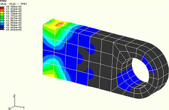
The equivalent plastic strain in a material (PEEQ) is a scalar variable that is used to represent the material's inelastic deformation. If this variable is greater than zero, the material has yielded. Those parts of the lug that have yielded can be identified in a contour plot of PEEQ by selecting Result![]() Field Output from the main menu bar and selecting PEEQ from the list of output variables in the dialog box that appears. Set the minimum contour limit to a very small magnitude (1.E-6) of equivalent plastic strain by bringing up the Contour Plot Options dialog box. Thus, any areas in the model plotted in dark blue in ABAQUS/Viewer still have elastic material behavior (see Figure 8–12).
Field Output from the main menu bar and selecting PEEQ from the list of output variables in the dialog box that appears. Set the minimum contour limit to a very small magnitude (1.E-6) of equivalent plastic strain by bringing up the Contour Plot Options dialog box. Thus, any areas in the model plotted in dark blue in ABAQUS/Viewer still have elastic material behavior (see Figure 8–12).
Creating a variable-variable (stress-strain) plot
The X–Y plotting capability in ABAQUS/Viewer was introduced in Chapter 7, “Nonlinearity.” In this section you will learn how to create X–Y plots showing the variation of one variable as a function of another. You will create a stress-strain plot for one of the integration points in an element adjacent to the constrained end of the lug. You saved the stress and strain data needed for this plot in the output database (.odb) file; therefore, use the following procedure to create X–Y plots in ABAQUS/Viewer.
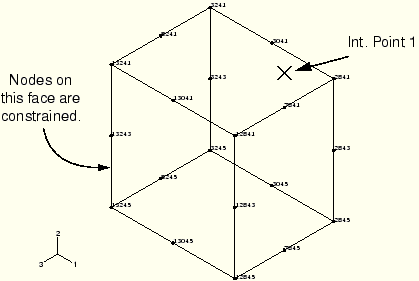
In the model used in this discussion, the stress-strain data were saved for element 206. You may have specified a different element number in your model; if you did, use that element number in place of 206 in the input examples that follow. Also, use data from an integration point that is closest to the top surface of the lug but not adjacent to the constrained nodes. In the model discussed here, integration point 1 satisfies these requirements, as shown in Figure 8–13.
To create history curves of stress and direct strain along the lug in element 206:
From the main menu bar, select Result![]() History Output.
History Output.
The History Output dialog box appears.
Use the scroll bar in the Output Variables list to locate and select the MISES stress at element 206, integration point 1.
The Mises stress, rather than the component of the true stress tensor, is used because the plasticity model defines plastic yield in terms of Mises stress.
Click Save As to save the X–Y data.
The Save XY Data As dialog box appears.
Enter the name MISES, and click OK.
Use the scroll bar in the Output Variables list to locate and select the direct strain (E11) at the same integration point, and save it under the name E11.
This strain component is used because it is the largest component of the total strain tensor at this point; using it clearly shows the elastic, as well as the plastic, behavior of the material at this integration point.
Click Dismiss to close the History Output dialog box.
Each of the curves that you have created is a history (variable versus time) plot. You must combine these two plots, eliminating the time dependence, to produce the desired stress-strain plot.
To combine history curves to produce a stress-strain plot:
From the main menu bar, select Tools![]() XY Data
XY Data![]() Create.
Create.
The Create XY Data dialog box appears.
Select Operate on XY data, and click Continue.
The Operate on XY data dialog box appears.
From the Operators listed, select combine(X,X).
combine( ) appears in the text field at the top of the dialog box.
In the XY Data field, drag the cursor across E11 and MISES to select both data objects.
Click Add to Expression. The expression combine(“E11”, “MISES”) appears in the text field. In this expression “E11” will determine the X-values and “MISES” will determine the Y-values in the combined plot.
Save the combined data object by clicking Save As at the bottom of the dialog box.
The Save XY Data As dialog box appears. In the Name text field, type SVE11; and click OK to close the dialog box.
To view the combined stress-strain plot, click Plot Expression at the bottom of the dialog box.
Click Cancel to close the dialog box.
This X–Y plot would be clearer if the limits on the X- and Y-axes were changed. Use the XY Plot Options in ABAQUS/Viewer to do this.
To customize the stress-strain curve:
Click XY Plot Options in the prompt area.
The XY Plot Options dialog box appears.
Set the maximum range of the X-axis (E11) to 0.07 strain, the maximum range of the Y-axis (MISES) to 500 MPa stress, and the minimum stress to 0.0 MPa.
Click OK to close the dialog box.
It will also be helpful to display a symbol at each data point of the curve. Click XY Curve Options in the prompt area.
The XY Curve Options dialog box appears.
From the XY Data field, select the stress-strain curve (SVE11).
The SVE11 data object is highlighted.
Toggle on Show symbol. Accept the defaults, and click OK at the bottom of the dialog box.
The stress-strain plot appears with a symbol at each data point of the curve.
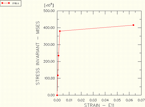
You should now have a plot similar to the one shown in Figure 8–14.
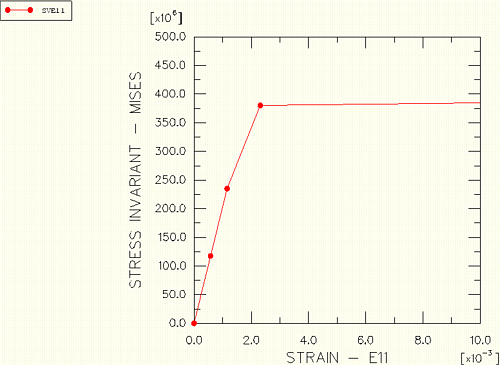
The stress-strain curve shows that the material behavior was linear elastic for this integration point during the first two increments of the simulation. In this plot it appears that the material remains linear during the third increment of the analysis; however, it does yield during this increment. This illusion is created by the extent of strain shown in the plot. If you limit the maximum strain displayed to 0.01 and set the minimum value to 0.0, the nonlinear material behavior in the third increment can be seen more clearly (see Figure 8–15). This stress-strain curve contains another apparent error. It appears that the material yields at 250 MPa, which is well below the initial yield stress. However, this error is caused by the fact that ABAQUS/Viewer connects the data points on the curve with straight lines. If you limit the increment size, the additional points on the graph will provide a better display of the material response and show yield occurring at exactly 380 MPa.The results from this second simulation indicate that the lug will withstand this 60 kN load if the steel hardens after it yields. Taken together, the results of the two simulations demonstrate that it is very important to determine the actual post-yield hardening behavior of the steel. If the steel has very little hardening, the lug may collapse under the 60 kN load. Whereas if it has moderate hardening, the lug will probably withstand the load although there will be extensive plastic yielding in the lug (see Figure 8–12). However, even with plastic hardening, the factor of safety for this loading will probably be very small.