This example is a continuation of the linear skew plate simulation described in Chapter 5, “Using Shell Elements,” and shown in Figure 7–11.
Having already simulated the linear response of the plate, you will now reanalyze it including the effects of geometric nonlinearity. The results from the linear simulation indicated that nonlinear effects may be important for this problem. With the results of this analysis, you will now be able to judge whether this is true or not.You only need to modify the history data to convert this model from a linear simulation to a nonlinear simulation.
Copy the input file skew.inp to skew_nl.inp, and incorporate the changes described below. If you wish to create the entire model using ABAQUS/CAE please refer to “Example: nonlinear skew plate,” Section 8.4 of Getting Started with ABAQUS.
Add the NLGEOM parameter to the *STEP option, and remove the PERTURBATION parameter. This indicates that the analysis now includes nonlinear geometric effects. The default maximum number of increments is 100; ABAQUS may use fewer increments than this upper limit, but it will stop the analysis if it needs more.
Your modified *STEP option should look like:
*STEP, NLGEOM
You may also wish to modify the description of the step to reflect that this is now a nonlinear analysis.
Defining the step time
You need to add a data line to the *STATIC option to specify the size of the initial time increment, ![]() , for the analysis and the total step time for the simulation. Use a total step time of 1.0, and specify
, for the analysis and the total step time for the simulation. Use a total step time of 1.0, and specify ![]() such that ABAQUS applies 10% of the load in the first increment. The completed *STATIC option block will, therefore, be
such that ABAQUS applies 10% of the load in the first increment. The completed *STATIC option block will, therefore, be
*STATIC
0.1,1.0
Output control
In a linear analysis ABAQUS solves the equilibrium equations once and calculates the results for this one solution. A nonlinear analysis can produce much more output because results can be requested at the end of each converged increment. If you do not select the output requests carefully, the output files become very large, potentially filling the disk space on your computer.
As noted earlier, output is available in four different files:
the output database (.odb) file, which contains data in a neutral binary format necessary to postprocess the results with ABAQUS/Viewer;
the data (.dat) file, which contains printed tables of selected results;
the restart (.res) file, which is used to continue the analysis; and
the results (.fil) file, which is used with third-party postprocessors.
The options for restart and results file output will not be discussed here. If selected carefully, data can be saved frequently during the simulation without using excessive disk space.
Remove the existing output requests from your input file; and add the following output options, which ensure that only selected output is saved during the nonlinear analysis.
To reduce the size of the output database file, use the FREQUENCY parameter on the *OUTPUT, FIELD option; in this simulation you should write field output every second increment. Thus, set the FREQUENCY parameter equal to 2 on the *OUTPUT option:
*OUTPUT, FIELD, FREQUENCY=2, VARIABLE=PRESELECTThe parameter VARIABLE=PRESELECT indicates that a preselected set of the most commonly used field variables for a given type of analysis will be written to the output database (.odb) file. If you are simply interested in the final results, set the FREQUENCY parameter equal to a large number. Results are always stored at the end of each step, regardless of the value of the FREQUENCY parameter; therefore, using a large value causes only the final results to be saved.
Request that the displacements of the nodes at the midspan be saved to the output database file. These results will be used later to demonstrate the X–Y plotting capability in ABAQUS/Viewer. Use the default FREQUENCY value (FREQUENCY=1) for this history output request for the output database file. Here the *NODE OUTPUT option must appear immediately after the history output request. Remember to use the NSET or ELSET parameters when limiting the output being requested to a subset of the model; otherwise, the default subset, which is the entire model, will be used.
Finally, request that reaction forces (RF) be printed for all the nodes in the model and that the displacements (U) be printed for the nodes at the midspan (node set MIDSPAN). You will need two *NODE PRINT options because you are requesting results for two different subsets of the model. Again, use the FREQUENCY parameter to reduce the amount of output; print the data every second increment. Suppress the printing of all element results by using *EL PRINT, FREQUENCY=0. To suppress output on any output request option, set FREQUENCY=0 on the output request.
The new list of output request option blocks in your input file should look like:
*OUTPUT, FIELD, FREQUENCY=2, VARIABLE=PRESELECT
*OUTPUT, HISTORY, FREQUENCY=1
*NODE OUTPUT, NSET=MIDSPAN
U,
*NODE PRINT, NSET=MIDSPAN, FREQUENCY=2
U,
*NODE PRINT, SUMMARY=NO, TOTALS=YES, FREQUENCY=2
RF,
*EL PRINT, FREQUENCY=0
Finally, complete the step definition by using the *END STEP option.
*END STEP
Store the modified input in a file called skew_nl.inp (an example input file is listed in “Nonlinear skew plate,” Section A.5). Run the analysis using the following command:
abaqus job=skew_nl interactive
During a nonlinear analysis, two additional output files become very important. They are the status file (skew_nl.sta) and the message file (skew_nl.msg). As the analysis progresses, ABAQUS will write data to both of these files. You can view the data even as ABAQUS continues your analysis. You will need to learn how to use the data in these files to assess ABAQUS's progress on your simulations. There may be situations where you decide, based on information in these files, to terminate your analysis early. A more likely scenario is that you may need to use these files to learn what caused ABAQUS to terminate your analysis prematurely; i.e., what caused the convergence problems.
Status file
The status file is particularly useful for monitoring the progress of a nonlinear simulation while the job is running. The output below shows the status file for this nonlinear skewed plate example.
 SUMMARY OF JOB INFORMATION:
 STEP  INC ATT SEVERE EQUIL TOTAL  TOTAL      STEP       INC OF       DOF    IF
               DISCON ITERS ITERS  TIME/    TIME/LPF    TIME/LPF    MONITOR RIKS
               ITERS               FREQ
   1     1   1     0     4     4  0.100      0.100      0.1000
   1     2   1     0     2     2  0.200      0.200      0.1000
   1     3   1     0     2     2  0.350      0.350      0.1500
   1     4   1     0     3     3  0.575      0.575      0.2250
   1     5   1     0     3     3  0.913      0.913      0.3375
   1     6   1     0     2     2  1.00       1.00       0.08750
The status file contains a separate line for every converged increment in the simulation. The first column shows the step number—in this case there is only one step. The second column gives the increment number. The sixth column shows the number of iterations ABAQUS needed to obtain a converged solution in each increment; for example, ABAQUS needed 4 iterations in increment 1. The eighth column shows the total step time completed, and the ninth column shows the increment size (This example shows how ABAQUS automatically controls the increment size and, therefore, the proportion of load applied in each increment. In this analysis ABAQUS applied 10% of the total load in the first increment: you specified ![]() to be 0.1 and the step time to be 1.0. ABAQUS needed four iterations to converge to a solution in the first increment. ABAQUS only needed two iterations in the second increment, so it automatically increased the size of the next increment by 50% to
to be 0.1 and the step time to be 1.0. ABAQUS needed four iterations to converge to a solution in the first increment. ABAQUS only needed two iterations in the second increment, so it automatically increased the size of the next increment by 50% to ![]() = 0.15. ABAQUS also increased
= 0.15. ABAQUS also increased ![]() in both the fourth and fifth increments. It adjusted the final increment size to be just enough to complete the analysis; in this case the final increment size was 0.0875.
in both the fourth and fifth increments. It adjusted the final increment size to be just enough to complete the analysis; in this case the final increment size was 0.0875.
Message file
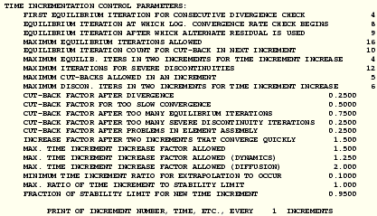
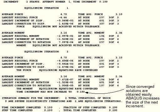
The message file contains more detailed information about the progress of the analysis than the status file. ABAQUS lists all of the tolerances and parameters to control the analysis at the start of each step in the message file. This is done for each step because these controls can be modified from step to step. The default values of these controls are appropriate for most analyses, so normally it is not necessary for you to modify them. The modification of control tolerances and parameters is beyond the scope of this guide (it is discussed in “Commonly used control parameters,” Section 8.3.2 of the ABAQUS Analysis User's Manual).

ABAQUS lists a summary of each iteration in the message file after the lists of tolerances and controls. It prints the values of the largest residual force, ![]() ; largest increment of displacement,
; largest increment of displacement, ![]() ; the largest correction to displacement,
; the largest correction to displacement, ![]() ; and the time averaged force,
; and the time averaged force, ![]() . It also prints the nodes and degrees of freedom (dof) at which
. It also prints the nodes and degrees of freedom (dof) at which ![]() ,
, ![]() , and
, and ![]() occur. A similar summary is printed for rotational degrees of freedom.
occur. A similar summary is printed for rotational degrees of freedom.
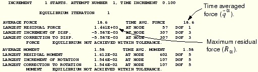
In this example the initial time increment is 0.1 seconds, as specified in the input file. The average force for the increment is 18.6 N, and ![]() has the same value since this is the first increment. The largest residual force in the model,
has the same value since this is the first increment. The largest residual force in the model, ![]() , is 1461 N, which is clearly greater than 0.005 ×
, is 1461 N, which is clearly greater than 0.005 × ![]() .
. ![]() occurred at node 57 in degree of freedom 1. ABAQUS must also check for equilibrium of the moments in the model since this model includes shell elements. The moment/rotation field also failed to satisfy the equilibrium check.
occurred at node 57 in degree of freedom 1. ABAQUS must also check for equilibrium of the moments in the model since this model includes shell elements. The moment/rotation field also failed to satisfy the equilibrium check.
Although failure to satisfy the equilibrium check is enough to cause ABAQUS to try another iteration, you should also examine the displacement correction. In the first iteration of the first increment of the first step the largest increment of displacement, ![]() , and the largest correction to displacement,
, and the largest correction to displacement, ![]() , are both –5.587 × 10⁻³ m; and the largest increment of rotation and correction to rotation are both 1.546 × 10⁻² radians. Since the incremental values and the corrections are always equal in the first iteration of the first increment of the first step, the check that the largest corrections to nodal variables are less than 1% of the largest incremental values will always fail. However, if ABAQUS judges the solution to be linear (a judgement based on the magnitude of the residuals,
, are both –5.587 × 10⁻³ m; and the largest increment of rotation and correction to rotation are both 1.546 × 10⁻² radians. Since the incremental values and the corrections are always equal in the first iteration of the first increment of the first step, the check that the largest corrections to nodal variables are less than 1% of the largest incremental values will always fail. However, if ABAQUS judges the solution to be linear (a judgement based on the magnitude of the residuals, ![]() < 10–8
< 10–8![]() ), it will ignore this criterion.
), it will ignore this criterion.
Since ABAQUS did not find an equilibrium solution in the first iteration, it tries a second iteration.
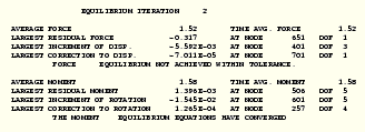
In the second iteration ![]() has fallen to –0.317 N at node 651 in degree of freedom 1. However, equilibrium is not satisfied in this iteration because 0.005
has fallen to –0.317 N at node 651 in degree of freedom 1. However, equilibrium is not satisfied in this iteration because 0.005 ![]() , where
, where ![]() = 1.52 N, is still less than
= 1.52 N, is still less than ![]() . The displacement correction criterion also failed again because
. The displacement correction criterion also failed again because ![]() = –7.011 × 10⁻⁵, which occurred at node 701 in degree of freedom 1, is more than 1% of
= –7.011 × 10⁻⁵, which occurred at node 701 in degree of freedom 1, is more than 1% of ![]() = –5.592 × 10⁻³, the maximum displacement increment.
= –5.592 × 10⁻³, the maximum displacement increment.
Both the moment residual check and the largest correction to rotation check were satisfied in this second iteration; however, ABAQUS must perform another iteration because the solution did not pass the force residual check (or the largest correction to displacement criterion). The message file summaries for the additional iterations necessary to obtain a solution in the first increment are shown below.
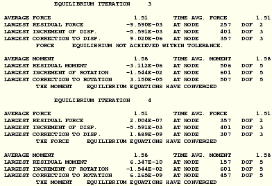
After four iterations ![]() = 1.51 N and
= 1.51 N and ![]() = 2.004 × 10⁻⁷ N at node 357 in degree of freedom 2. These values satisfy
= 2.004 × 10⁻⁷ N at node 357 in degree of freedom 2. These values satisfy ![]() < 0.005 ×
< 0.005 × ![]() , so the force residual check is satisfied. Comparing
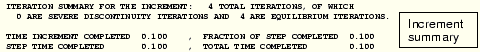
, so the force residual check is satisfied. Comparing ![]() to the largest increment of displacement shows that the displacement correction is below the required tolerance. The solution for the forces and displacements has, therefore, converged. The checks for both the moment residual and the rotation correction continue to be satisfied, as they have been since the second iteration. With a solution that satisfies equilibrium for all variables (displacement and rotation in this case), the first load increment is complete. The increment summary shows the number of iterations that were required for this increment, the size of the increment, and the fraction of the step that has been completed.
to the largest increment of displacement shows that the displacement correction is below the required tolerance. The solution for the forces and displacements has, therefore, converged. The checks for both the moment residual and the rotation correction continue to be satisfied, as they have been since the second iteration. With a solution that satisfies equilibrium for all variables (displacement and rotation in this case), the first load increment is complete. The increment summary shows the number of iterations that were required for this increment, the size of the increment, and the fraction of the step that has been completed.
The second increment requires two iterations to converge.
ABAQUS continues this process of applying an increment of load then iterating to find a solution until it completes the whole analysis (or reaches the increment specified as the value of the INC parameter). In this analysis it required four more increments. ABAQUS gives a summary at the end of the message file of how the analysis progressed and how many error and warning messages it issued. The summary for this analysis is shown below. An important item to check is how many iterations ABAQUS uses. In this analysis it performed 16 iterations over the six increments: the model's system of equations was solved 16 times (i.e., 16 matrix decompositions), illustrating the increased computational expense of nonlinear analyses compared with linear simulations.
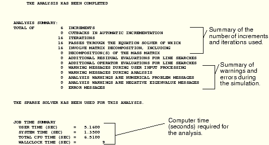
You should always check this summary at the end of every ABAQUS simulation. It tells you if the analysis job ran to completion (i.e., whether it terminated without a FORTRAN error), and it gives the number of error and warning messages ABAQUS issued during the simulation. Always investigate any errors or warnings. All warnings and errors generated during the analysis are found in the message (.msg) file. Warnings issued “during user input processing” are found in the data (.dat) file.
Data file
The tables of displacements and reaction forces that you requested are in the data (.dat) file. The midspan deflections at the end of the step can be found near the end of the file.
   THE FOLLOWING TABLE IS PRINTED FOR NODES BELONGING TO NODE SET MIDSPAN

    NODE FOOT-   U1          U2          U3          UR1         UR2         UR3
         NOTE

     351      -2.6632E-03 -7.4371E-04 -4.9226E-02
     353      -2.5267E-03 -7.5635E-04 -4.8088E-02
     355      -2.4189E-03 -7.7812E-04 -4.6726E-02
     357      -2.2649E-03 -7.9809E-04 -4.5314E-02

 MAXIMUM      -2.2649E-03 -7.4371E-04 -4.5314E-02  0.0000E+00  0.0000E+00  0.0000E+00
 AT NODE         357         351         357           0           0           0

 MINIMUM      -2.6632E-03 -7.9809E-04 -4.9226E-02  0.0000E+00  0.0000E+00  0.0000E+00
 AT NODE         351         357         351           0           0           0
Compare these with the displacements from the linear analysis in Chapter 5, “Using Shell Elements.” The maximum displacement at the midspan in this simulation is about 9% less than that predicted from the linear analysis. Including the nonlinear geometric effects in the simulation reduces the vertical deflection (U3) of the midspan of the plate.
Another difference between the two analyses is that in the nonlinear simulation there are nonzero deflections in the 1- and 2-directions. What effects make the in-plane displacements, U1 and U2, nonzero in the nonlinear analysis? Why is the vertical deflection of the plate less in the nonlinear analysis?
The plate deforms into a curved shape: a geometry change that is taken into account in the nonlinear simulation. As a consequence, membrane effects cause some of the load to be carried by membrane action rather than by bending alone. This makes the plate stiffer. In addition, the pressure loading, which is always normal to the plate's surface, starts to have a component in the 1- and 2-directions as the plate deforms. The nonlinear analysis includes the effects of this stiffening and the changing direction of the pressure. Neither of these effects is included in the linear simulation.
The differences between the linear and nonlinear simulations are sufficiently large to indicate that a linear simulation is not adequate for this plate under this particular loading condition.
For five degree of freedom shells, such as the S8R5 element used in this analysis, ABAQUS does not output total rotations at the nodes.
When you are in the directory containing the output database file skew_nl.odb, type the command
abaqus viewer odb=skew_nlat the operating system prompt.
Showing the available frames
To begin this exercise, determine the available output frames (the increment intervals at which results were written to the output database).
To show the available frames:
From the main menu bar, select Result![]() Step/Frame.
Step/Frame.
The Step/Frame dialog box appears.
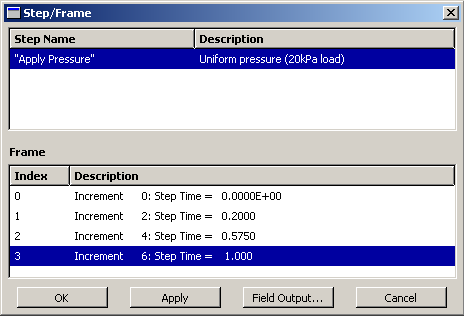
During the analysis ABAQUS wrote field output results to the output database file every second increment (since the command *OUTPUT, FIELD, FREQUENCY=2, VARIABLE=PRESELECT was in the input file). ABAQUS/Viewer displays the list of the available frames, as shown in Figure 7–12.
The list tabulates the steps and increments for which field variables are stored. This analysis consisted of a single step with six increments. The results for increment 0 (the initial state of the step) are saved by default and you saved data for increments 2, 4, and 6. By default, ABAQUS/Viewer always uses the data for the last available increment saved on the output database file.
Click OK to dismiss the Step/Frame dialog box.
Displaying the deformed and undeformed model shapes
You will now display the deformed and undeformed model shapes together.
To superimpose the undeformed model shape on the deformed model shape:
From the main menu bar, select Plot![]() Deformed Shape; or use the
Deformed Shape; or use the ![]() tool in the toolbox.
tool in the toolbox.
ABAQUS/Viewer displays the deformed model shape at the end of the analysis.
From the main menu bar, select Options![]() Deformed Shape.
Deformed Shape.
ABAQUS/Viewer displays the Deformed Shape Plot Options dialog box.
Click the Basic tab if it is not already selected, and toggle on Superimpose undeformed plot.
Click OK to apply your changes and to close the dialog box.
Changing the view
You can change the default isometric view using the options in the View menu or the view tools in the toolbar.
To rotate the view:
From the main menu bar, select View![]() Rotate; or use the
Rotate; or use the ![]() tool from the toolbar.
tool from the toolbar.
Drag the mouse over the virtual trackball in the viewport.
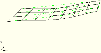
The view rotates interactively. Move the mouse, with mouse button 1 depressed, to obtain a view similar to that shown in Figure 7–13.
Click mouse button 2 in the viewport or the ![]() tool from the toolbar to exit the rotation mode.
tool from the toolbar to exit the rotation mode.
Using results from other frames
You can evaluate the results from other increments saved to the output database file by selecting the appropriate frame.
To select a new frame:
From the main menu bar, select Result![]() Step/Frame.
Step/Frame.
The Step/Frame dialog box appears.
Select Increment 4 from the Frame menu.
Click OK to apply your changes and to close the Step/Frame dialog box.
Any plots now requested will use results from increment 4. Repeat this procedure, substituting the increment number of interest, to move through the output database file.
X–Y plotting
You saved the displacements of the midspan nodes (node set MIDSPAN) in the history portion of the output database file skew_nl.odb for each increment of the simulation. You can use these results to create X–Y plots.
To create X–Y plots of the midspan displacements:
From the main menu bar, select Result![]() History Output.
History Output.
ABAQUS/Viewer displays the History Output dialog box. To see the complete description of the variable choices, increase the width of the History Output dialog box by dragging the right or left edge.
The Output Variables field contains a list of all the variables in the history portion of the output database; these are the only history output variables you can plot. Select (using [Ctrl]+Click) the vertical motion of both node 351 (Spatial displacement: U3 at Node 351 in NSET MIDSPAN) and node 357 (Spatial displacement: U3 at Node 357 in NSET MIDSPAN).
Click Plot.
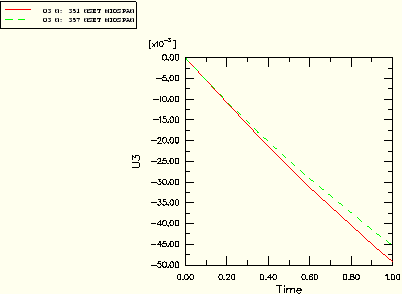
ABAQUS reads the data for both curves from the output database file and plots a graph similar to the one shown in Figure 7–14. (For clarity, the second curve has been changed to a dashed line.)
The nonlinear nature of this simulation is clearly seen in these curves: as the analysis progresses, the plate stiffens. The effects of geometric nonlinearity mean that a structure's stiffness changes as it deforms. In this simulation the plate deforms as it gets stiffer due to membrane effects. Therefore, the resulting peak displacement is less than that predicted by the linear analysis, which did not include this effect.
You can create X–Y curves from either history or field data stored in the output database (.odb) file. X–Y curves can also be read from an external file or they can be typed into ABAQUS/Viewer interactively. Once curves have been created, their data can be further manipulated and plotted to the screen in graphical form.
The X–Y plotting capability of ABAQUS/Viewer is discussed further in Chapter 8, “Materials.”